How to Plot Logistic Regression’s Decision Boundary?

1. Introduction

In this tutorial, we’ll show how to plot the decision boundary of a logistic regression classifier. We’ll focus on the binary case with two classes we usually call positive and negative. We’ll also assume that all the features are continuous.

2. Decision Boundary

Let $\mathcal{X}$ be the space of objects we want to classify using machine learning. The decision boundary of a classifier is the subset of $\boldsymbol{\mathcal{X}}$ containing the objects for which the classifier’s score is equal to its decision threshold.

In the case of logistic regression (LR), the score $f(x)$ of an object $x$ is the estimate of the probability that $x$ is positive, and the decision threshold is 0.5:

$\{ x \in \mathcal{X} \mid f(x) = 0.5 \}$

Visualizing the boundary helps us understand how our classifier works and compare it to other classification models.

3. Plotting the Boundary

To plot the boundary, we first have to find its equation.

3.1. The Boundary Equation

We can derive the equation of the decision boundary by plugging in the formula of LR into the condition $f(x) = 0.5$ .

We’ll assume that $x= [x_0, x_1, x_2, \ldots, x_n]^T$ is an $(n+1) \times 1$ vector with $x_0=1$ to make the LR equation more compact. In preprocessing, we can always prepend $x_0=1$ to any $n$ -dimensional $x$ .

Consequently, we have:

$f(x) = \frac{1}{1 + e^{-\theta x}} = \frac{1}{2}$

where $\theta = [\theta_1, \theta_2, \ldots, \theta_n]^T$ is the $(n+1) \times 1$ parameter vector of our LR model $f$ . From there, we get:

$\begin{aligned} \frac{1}{1 + e^{-\theta^T x}} &= \frac{1}{2} \\ 1 + e^{-\theta^T x} &= 2 \\ e^{-\theta^T x} &= 1 \\ - \theta^T x &= 0 \\ \theta^T x &= 0 \\ \sum_{i=0}\theta_i x_i &= 0 \end{aligned}$

3.2. The Shape of the Boundary in Two and Three Dimensions

If $n=2$ , the boundary equation becomes:

$\theta_0 + \theta_1 x_1 + \theta_2 x_2 = 0$

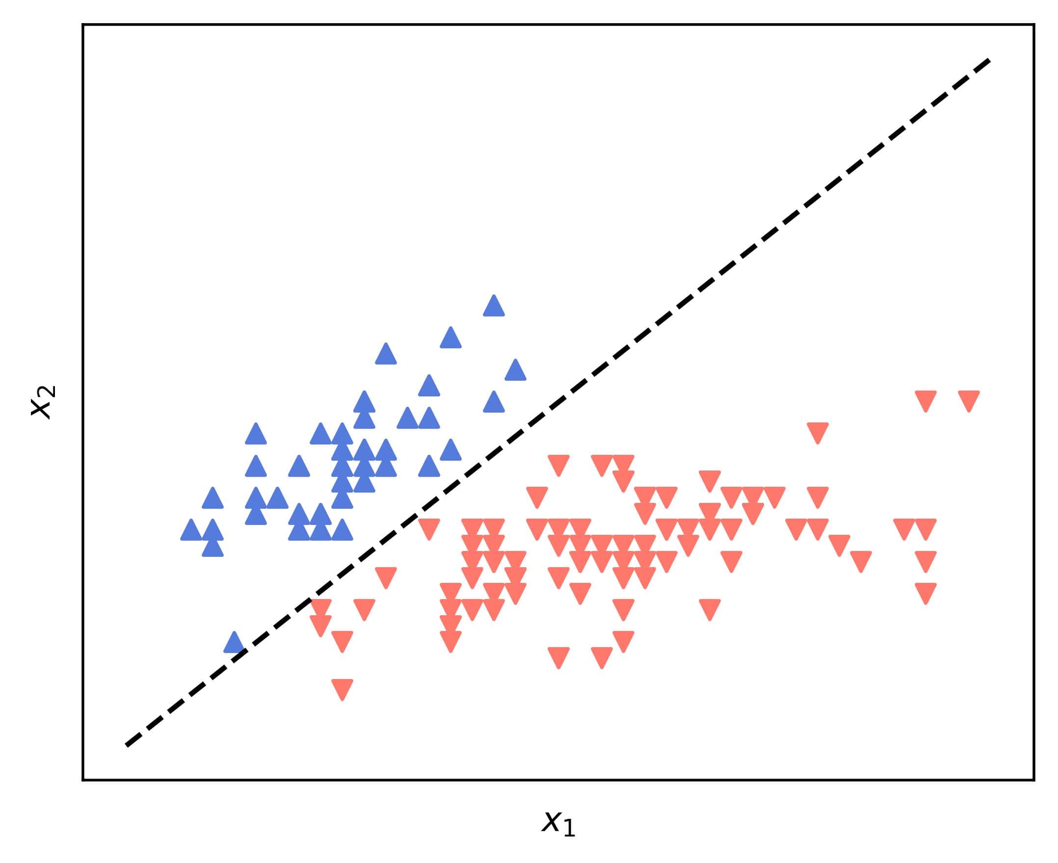
That’s a line in the $(x_1, x_2$ ) plane. For example, if we use the iris dataset with $x_1$ and $x_2$ being the sepal length and width, and with versicolor and virginica classes blended into one, we’ll get a straight line:

We don’t have to consider the degenerate case where $\theta_0=\theta_1=\theta_2=0$ . That implies that no features of $x$ are used, so we won’t use such a model anyway. Let’s say $\theta_2 \neq 0$ . The explicit boundary’s equation is then:

$x_2 = -\frac{\theta_1}{\theta_2}x_1 - \frac{\theta_0}{\theta_2}$

If $n=3$ , we have a plane given by:

$\theta_0 + \theta_1 x_1 + \theta_2 x_2 + \theta_3 x_3 = 0$

Let $\theta_3 \neq 0$ . Then, we can write the equation in the explicit form:

$x_3 = -\frac{\theta_2}{\theta_3} x_2 -\frac{\theta_1}{\theta_3}x_1 - \frac{\theta_0}{\theta_3}$

3.3. Algorithm

We can use any plotting tool to visualize lines and planes corresponding to these equations. If we have to do it from scratch, we can iterate over the independent features in small increments and calculate the dependent feature using the explicit forms:

The limits $l$ and $u$ determine the part of the boundary we want to focus on.

3.4. The Limits of Visualization

We have two questions at his point:

Can we visualize a boundary in multiple dimensions?
Is a boundary always a line or a plane?

Let’s find out.

4. Multiple Dimensions

If our objects have more than three features, we can visualize only the boundary’s projections onto the planes and spaces defined by pairs and triplets of features.

One way we deal with this is to choose the features for visualization and keep the others at constant values, such as means or constants of interest we know from theory. Values that mean “the feature is absent or neutral” can also be helpful. In most, but not all cases, that would mean setting those other features to zeros.

4.1. Example

With 10 features $x_1, x_2, \ldots, x_{10}$ , we have $\binom{10}{2}=45$ feature pairs. Let’s say we choose $x_1$ and $x_2)$ for visualizing the boundary. In that case, we set $x_3, x_4, \ldots, x_10$ to some constant values. Let them be $x_3 = \chi_3, x_4 = \chi_4, \ldots, x_{10}=\chi_{10}$ .

Then, $\sum_{i = 3}^{10} \theta_i \chi_i$ is another constant. We add it to $\theta_0$ and proceed as if $x_1$ and $x_2$ are the only two features of interest:

$x_2 = -\frac{\theta_1}{\theta_2} - \frac{1}{\theta_2}\left(\theta_0 + \sum_{i = 3}^{10} \theta_i \chi_i \right)$

This can work for any pair or triplet of $x_1, x_2, \ldots, x_n$ .

However, a disadvantage of this approach is that the boundary depends on the chosen constants $\chi_i$ .

5. Curvatures

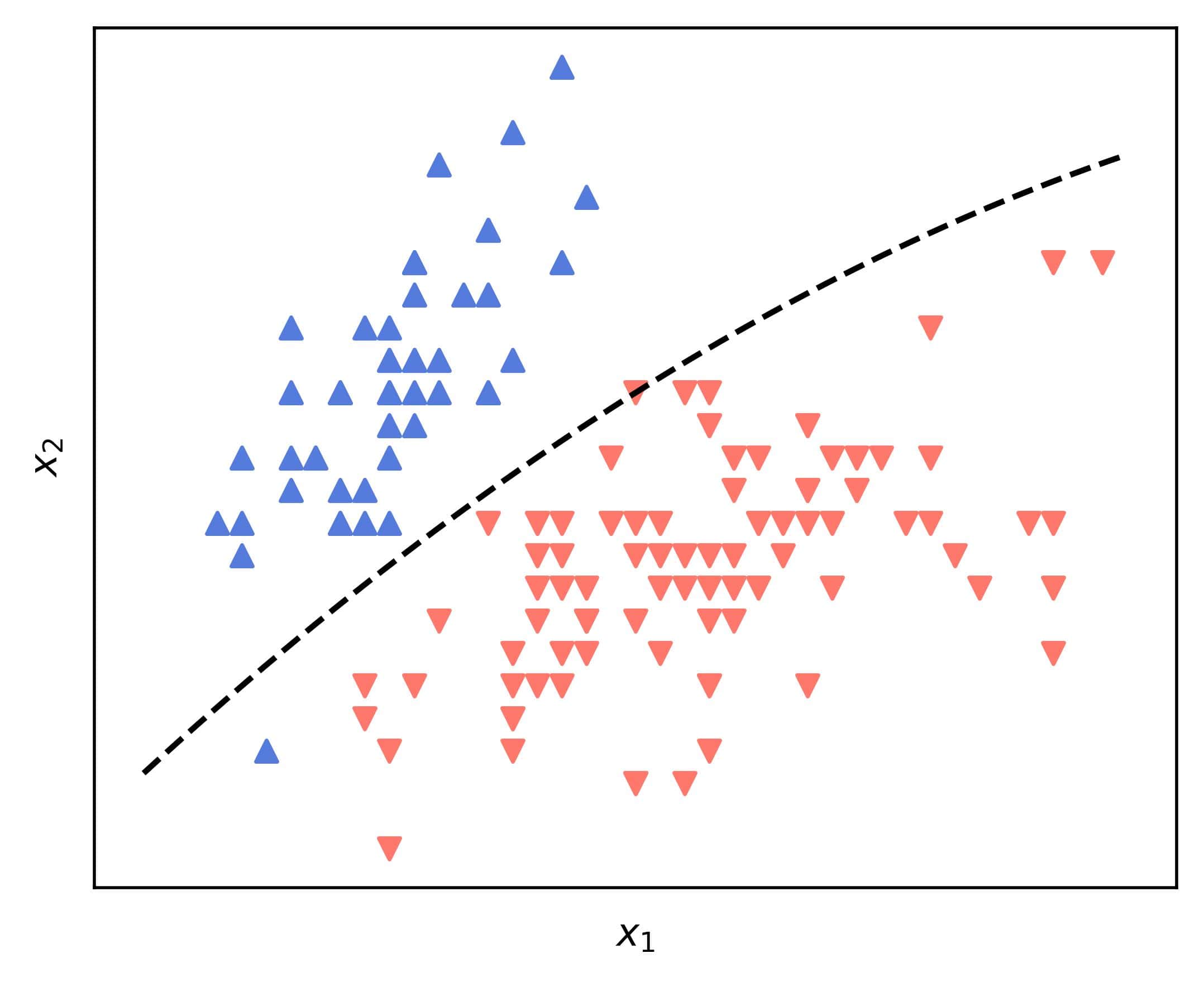
We can introduce curvatures with feature engineering.

Let’s say that our original features are $[x_1, x_2]$ . Before pretending $x_0 = 1$ , we can add $x_3=x_1^2$ . Then, the decision boundary becomes:

$\theta_0 + \theta_1 x_1 + \theta_2 x_2 + \theta_3 x_1^2 = 0 \implies x_2 = -\frac{\theta_0}{\theta_2} - \frac{\theta_1}{\theta_2}x_1 - \frac{\theta_3}{\theta_2}x_1^2$

which is a curve in the original $(x_1, x_2)$ space. For instance:

However, the same boundary is a plane in the augmented $(x_1, x_2, x_3)$ space.

6. Conclusion

In this article, we showed how to visualize the logistic regression’s decision boundary. Plotting it helps us understand how our logistic model works.

Core Concepts

Operating Systems

Neural Networks

Graph Theory

Latex

Full Archive

About Baeldung