

Learn through the super-clean Baeldung Pro experience:
>> Membership and Baeldung Pro.
No ads, dark-mode and 6 months free of IntelliJ Idea Ultimate to start with.
Learn through the super-clean Baeldung Pro experience:
>> Membership and Baeldung Pro.
No ads, dark-mode and 6 months free of IntelliJ Idea Ultimate to start with.
In computer graphics, the digital differential analyzer (DDA) algorithm is used to draw a line segment between two endpoints.
In this tutorial, we’ll explore the steps of the DDA algorithm in detail with an example. Furthermore, we’ll present the time and space complexity analysis. Finally, we’ll discuss the advantages and disadvantages of the DDA algorithm.
The DDA algorithm is part of the line drawing algorithms in computer graphics. Using the DDA algorithm, we can generate the intermediate points along a straight line between two given endpoints.
Now, let’s discuss how the DDA algorithm works. Considering the starting point  and ending point
  , first, we calculate the difference between the X-coordinates and Y-coordinates of the given points:
![\[difx = |X2 - X1|\]](/wp-content/ql-cache/quicklatex.com-f5c99850d8d466bc1a2c2358f278eef9_l3.svg "Rendered by QuickLaTeX.com")
![\[dify = |Y2- Y1|\]](/wp-content/ql-cache/quicklatex.com-6c1b3c288fa3ab0d2b35defc0ddb1fec_l3.svg "Rendered by QuickLaTeX.com")
Furthermore, the next step is to calculate the slope of the line to determine the direction of the next point:
![\[m = \frac{dify}{difx}\]](/wp-content/ql-cache/quicklatex.com-0505db71b87bd9a7136304bd9cfe1003_l3.svg "Rendered by QuickLaTeX.com")
Thus, if the slope value is positive  , we move towards an upward direction. On the other hand, if the slope value is negative
  , we progress towards a downward direction.
Furthermore, we calculate the total number of steps needed to reach the ending point from the starting point:
![\[S =max (difx, dify)\]](/wp-content/ql-cache/quicklatex.com-d45352efcaa91b43088956835720073a_l3.svg "Rendered by QuickLaTeX.com")
Now, let’s determine the value we need to increment for the X and Y axes for each step:
![\[Xins = \frac{difx}{S}\]](/wp-content/ql-cache/quicklatex.com-88a8453a84e9aeff223f379c15687184_l3.svg "Rendered by QuickLaTeX.com")
![\[Yins = \frac{dify}{S}\]](/wp-content/ql-cache/quicklatex.com-d083007cbd832e3311fcb5dddb49d57f_l3.svg "Rendered by QuickLaTeX.com")
Thus, starting from the initial point , we iterate through each step and increment the X and Y axis:
![\[X= X + Xins\]](/wp-content/ql-cache/quicklatex.com-d4c70d09b1da11c4ee5a773b529e2c5e_l3.svg "Rendered by QuickLaTeX.com")
![\[Y = Y + Yins\]](/wp-content/ql-cache/quicklatex.com-38241e6928730295c17eac2510fc7293_l3.svg "Rendered by QuickLaTeX.com")
Finally, rounding off is necessary when calculating the new points. As the pixel positions on a computer screen are discrete, we need to present them as integer numbers.
We know the steps of the DDA algorithm. Let’s take a look at the pseudocode:
algorithm DDA (X1, Y1, X2, Y2):
    difx = (|X2 - X1|)
    dify = (|Y2 - Y1|)
    s = max (difx, dify)
    Xins = difx / s
    Yins = dify / s
    X = X1
    Y = Y1
    while i <= s:
        X = X + Xins
        Y = Y + Yins
        Plot(Floor(X), Floor(Y))
        i = i + 1
Now, we examine the DDA algorithm’s computational complexity. The number of iterations we perform to find the intermediate X and Y points determines the time complexity of the DDA algorithm. In this case, the number of iterations is equal to  . Therefore, the overall time complexity of the DDA algorithm is
  .
.
Furthermore, let’s talk about the DDA algorithm’s space complexity. Typically, the space complexity depends on the variables and data structure used in the pseudocode. In this case, all the variables in the pseudocode occupy constant space. Additionally, we haven’t used any data structure that scales with the input size. Hence, we can conclude that the space complexity of the DDA algorithm is  .
.
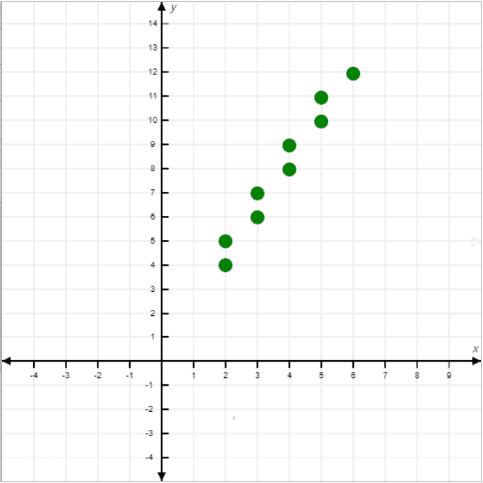
Let’s take an example where the starting point is (2, 4) and the ending point is (6, 12). Thus, we use the DDA algorithm to find the intermediate points.
First, we calculate  and
and  :
:
![\[difx = |6 - 2| = 4\]](/wp-content/ql-cache/quicklatex.com-580a0177b2efbbf8d9ff552267f21458_l3.svg "Rendered by QuickLaTeX.com")
![\[dify = |12 - 4| = 8\]](/wp-content/ql-cache/quicklatex.com-44de1e1aa436e329c17672efa0b75761_l3.svg "Rendered by QuickLaTeX.com")
Therefore, the total number of steps needed to reach the ending point is:
![\[s =max (difx, dify) = max (4, 8) = 8\]](/wp-content/ql-cache/quicklatex.com-cb98e188872c16bda0fdbc8eabf48986_l3.svg "Rendered by QuickLaTeX.com")
Furthermore, we calculate the value we need to increment for the X and Y axes for each step:
![\[Xins = \frac{difx}{S} = \frac{4}{8} = 0.5\]](/wp-content/ql-cache/quicklatex.com-d293f084763c3f8e555dd4cd1d6c6853_l3.svg "Rendered by QuickLaTeX.com")
![\[Yins = \frac{dify}{S} = \frac{8}{8} = 1\]](/wp-content/ql-cache/quicklatex.com-b30339c9cc6bd41de7c0fbd4dd5b663f_l3.svg "Rendered by QuickLaTeX.com")
Let’s calculate the intermediate points to draw a line between the start and end points:
| Number of iterations | X | Y | X + Xins | Y + Yins | (Floor(X), Floor(Y)) |
|---|---|---|---|---|---|
| 1 | 2 | 4 | 2 + 0.5 = 2.5 | 4 + 1 = 5 | (2,5) |
| 2 | 2.5 | 5 | 2.5 + 0.5 = 3 | 5 + 1 = 6 | (3,6) |
| 3 | 3 | 6 | 3 + 0.5 = 3.5 | 6 + 1 = 7 | (3,7) |
| 4 | 3.5 | 7 | 3.5 + 0.5 = 4 | 7 + 1 = 8 | (4,8) |
| 5 | 4 | 8 | 4 + 0.5 = 4.5 | 8 + 1 = 9 | (4,9) |
| 6 | 4.5 | 9 | 4.5 + 0.5 = 5 | 9 + 1 = 10 | (5,10) |
| 7 | 5 | 10 | 5 + 0.5 = 5.5 | 10 + 1 = 11 | (5,11) |
| 8 | 5.5 | 11 | 5.5 + 0.5 = 6 | 11 + 1 = 12 | (6,12) |
Finally, let’s plot all the points:
The DDA algorithm is commonly used for line drawing in computer graphics. Lines are fundamental graphics primitives. Hence, using a series of lines, we can generate complex graphics primitives, including rectangles, polygons, squares, grids, and different patterns.
Furthermore, we utilize the DDA algorithm in the computer-aided design (CAD) tool to generate 2D and 3D models. Additionally, some important computer graphics algorithms, such as image segmentation and edge detection, use the DDA algorithm.
Moreover, we also use the DDA algorithms in graphics editing software such as SuperPaint and Adobe Photoshop. Additionally, the line drawing process using the DDA algorithm is employed in simple animations and video games.
Now, let’s discuss some advantages as well as disadvantages of the DDA algorithm:
| Advantages | Disadvantages |
|---|---|
| Simple and easy to implement | Vulnerable to rounding errors |
| Faster than the other line drawing algorithms | Precision is limited |
| Efficient for basic 3D line-drawing tasks | Less efficient when dealing with vertical lines |
| Handle lines of varying steepness | Not suitable for drawing thick lines |
| Ideal when the number of pixels to be plotted is limited | Not ideal when the number of pixels to be plotted is significantly large |
In this article, we discussed the DDA algorithm in detail. We presented the pseudocode of the DDA algorithm with an example.
Finally, we explored the advantages and disadvantages of the DDA algorithm.