

Learn through the super-clean Baeldung Pro experience:
>> Membership and Baeldung Pro.
No ads, dark-mode and 6 months free of IntelliJ Idea Ultimate to start with.
Learn through the super-clean Baeldung Pro experience:
>> Membership and Baeldung Pro.
No ads, dark-mode and 6 months free of IntelliJ Idea Ultimate to start with.
In this tutorial, we’ll talk about Harris Corner Detection, a mathematical approach to detecting corners in an image. First, we’ll illustrate the mathematical formulation. Then, we’ll show the step-by-step procedure to perform the Harris Corner Detector.
A corner is a point whose local neighborhood is characterized by large intensity variation in all directions. Corners are important features in computer vision because they are points stable over changes of viewpoint and illumination. The so-called Harris Corner Detector was introduced by Chris Harris and Mike Stephens in 1988 in the paper “A Combined Corner and Edge Detector”.
Let’s consider a two-dimensional image  and a patch
  of size
  centered in
  . We want to evaluate the intensity variation occurred if the window is shifted by a small amount
  . Such variation can be estimated by computing the Sum of Squared Differences (SSD):
(1) ![\begin{equation*} \hbox{SSD}(u, v)=\sum_{\left(x, y)\right \in W} g(x,y) \left[I\left(x, y\right)-I\left(x+u, y+v\right)\right]^{2} \end{equation*}](/wp-content/ql-cache/quicklatex.com-e5d4afae4f083fc47f09d1fe8f8c24a5_l3.svg "Rendered by QuickLaTeX.com")
where  is a window function that can be a rectangular or a Gaussian function. We need to maximize the function
  for corner detection. Since
  and
and  are small, the shifted intensity
  can be approximated by the following first-order Taylor expansion:
(2) 
where  and
and  are partial derivatives of in
  and
and  direction, respectively. By substituting (2) in (1) we obtain:
(3) ![\begin{equation*} \hbox{SSD}(u, v) \approx \sum_{\left(x, y)\right \in W} g(x, y)\left[u^{2} I_{x}^{2}+2 u v I_{x} I_{y}+v^{2} I_{y}^{2}\right] . \end{equation*}](/wp-content/ql-cache/quicklatex.com-c19bf287f07688c042b27cf02c4c9b49_l3.svg "Rendered by QuickLaTeX.com")
The equation (3) can be expressed in the following matrix form:
(4) ![\begin{equation*} \hbox{SSD}(u, v) \approx\left[\begin{array}{ll} u & v \end{array}\right] M\left[\begin{array}{l} u \\ v \end{array}\right] \end{equation*}](/wp-content/ql-cache/quicklatex.com-6a1743d64a40a4090489993c1607fa32_l3.svg "Rendered by QuickLaTeX.com")
where  is a
is a  matrix computed from image derivatives:
(5) ![\begin{equation*} M=\sum_{\left(x, y)\right \in W}g(x, y)\left[\begin{array}{ll} I_{x} I_{x} & I_{x} I_{y} \\ I_{x} I_{y} & I_{y} I_{y} \end{array}\right] \end{equation*}](/wp-content/ql-cache/quicklatex.com-11af96f0ae425e7dfdfa94502e840c4b_l3.svg "Rendered by QuickLaTeX.com")
The matrix is called structure tensor.
The Harris detector uses the following response function that scores the presence of a corner within the patch:
(6) 
 is a constant to chose in the range
 ![[0.04, 0.06]](/wp-content/ql-cache/quicklatex.com-110b19ea7018536cb74ebadce0a2fbad_l3.svg "Rendered by QuickLaTeX.com") . Since is a symmetric matrix,
. Since is a symmetric matrix,  and
and  where
where  and
and  are the eigenvalues of . Hence, we can express the corner response as a function of the eigenvalues of the structure tensor:
(7) 
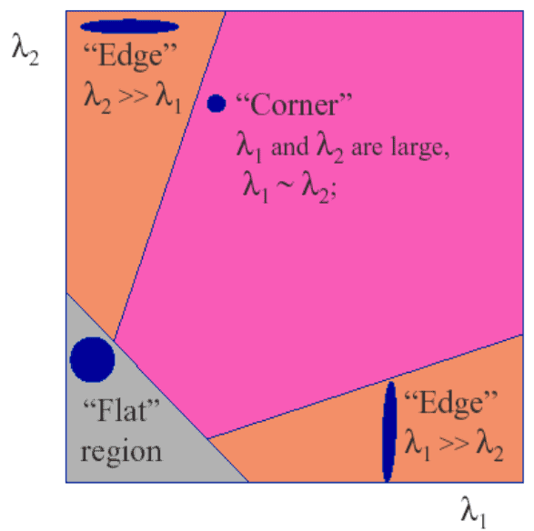
So the eigenvalues determine whether a region is an edge, a corner or flat:
and are small, then  is small and the region is flat;
 or viceversa, then
  and the region is an edge;
 and both eigenvalues are large, then R is large and the region is a corner.
The classification of the points using the eigenvalues of the structure tensor is represented in the following figure:
Harris corner detector consists of the following steps.
. The pixel values of are computed as a weighted sum of the corresponding  ,
,  ,
,  values:
(8) 
and by convolving the image with the Sobel operator:
(9) 
 ,
,  ,
,  . , , with a Gaussian filter or a mean filter. Define the structure tensor for each pixel as expressed in eq. (5).
 (10)
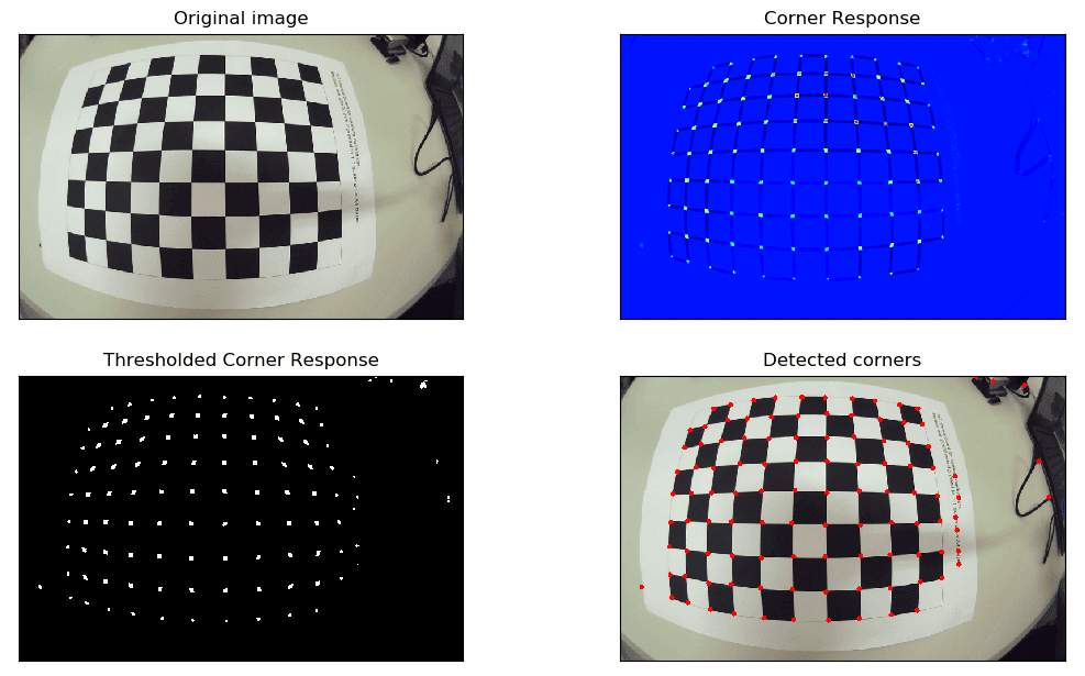
 on the value of and find pixels with responses above this threshold. Finally, compute the non-max suppression in order to pick up the optimal corners.
In the following figure we show a real application of the Harris Corner Detector. The corner response map (top-right image) was computed using Eq. 10 with k=0.04. The bottom-left image represents the thresholded corner response obtained with  . The detected corners obtained after the application of the non-max suppression are shown in the bottom-right image.
In this article, we reviewed the Harris Corner Detector, a fundamental technique in computer vision. We explained the mathematical formulation, and finally, we explained how to implement it.