Yes, we're now running our only Summer Sale. All Courses are 30% off until 20th July, 2026:
DBSCAN Clustering: How Does It Work?
Last updated: February 28, 2025

Learn through the super-clean Baeldung Pro experience:
>> Membership and Baeldung Pro.
No ads, dark-mode and 6 months free of IntelliJ Idea Ultimate to start with.
1. Introduction
In this tutorial, we’ll explain the DBSCAN (Density-based spatial clustering of applications with noise) algorithm, one of the most useful, yet also intuitive, density-based clustering methods.
We’ll start with a recap of what clustering is and how it fits into the machine learning domain. Then, we’ll describe the main concepts and steps taken in applying DBSCAN to a set of points. Finally, we’ll compare the clusters generated by the algorithm with clusters computed through two other popular methods: K-Means Clustering and HDBSCAN.
2. Clustering
To cluster a set of points is to assign each of them to a group based on the proximity to its neighbors. Each such group is called a cluster. The number of clusters heavily depends on both the number of points and how the points are spread out in space.
Naturally, clustering a set of points in 2D is very easy for humans, as it is clear to us that the next plot has 4 clusters:
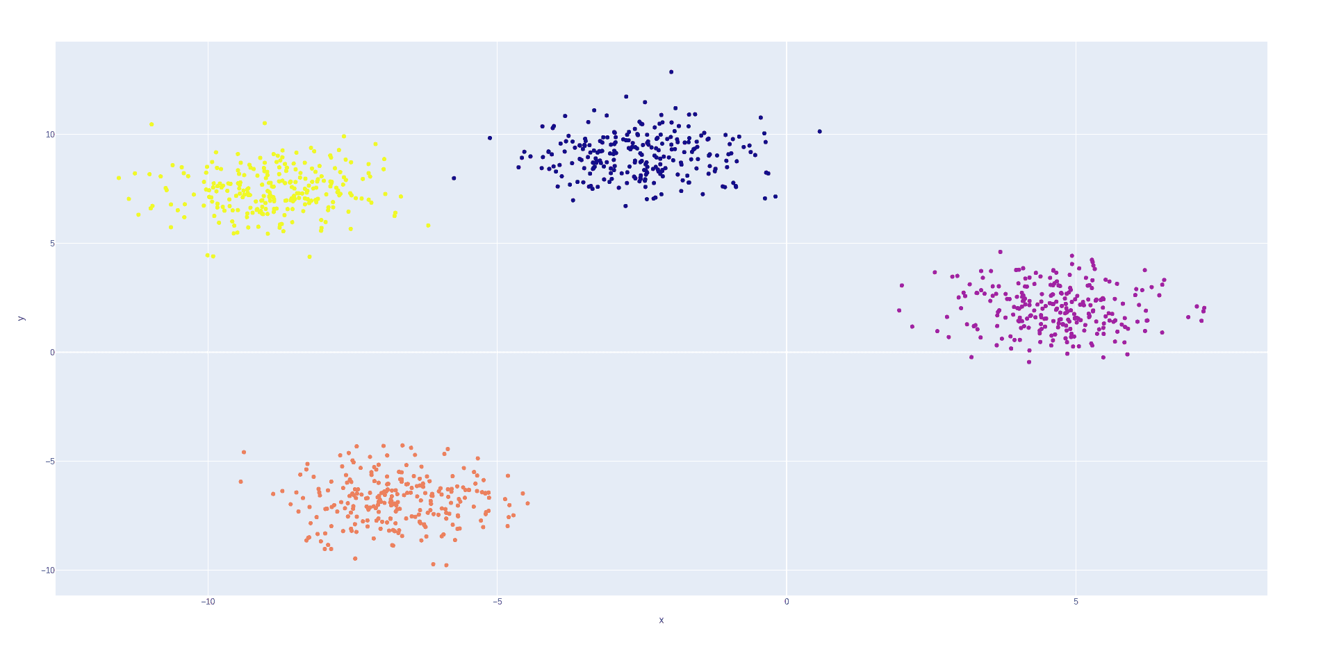
In fact, visualization is the most reliable way of judging if a clustering algorithm is performing well.
This, unfortunately, means that the situations in which these algorithms are most needed (points in more than 3 dimensions) are the hardest to evaluate. Other than the 2D and 3D case, it’s difficult to know if the algorithm really found the correct number of clusters.
However, by observing the performance of the algorithms in 2D we can get a clearer idea about their advantages and limitations.
2.1. Clustering Categories
There are 4 major categories of clustering algorithms:
- Centroid-based Clustering
- Density-based Clustering
- Distribution-based Clustering
- Hierarchical Clustering
Centroid-based clustering starts with a number of randomly positioned centroids (central points), which play the role of the centers of the found clusters. In a step-by-step fashion, these centroids are refined until they converge to the real centers of the clusters.
Density-based clustering groups are grouped up by the density of other points in their vicinity. Points that are really close together will form a cluster, while isolated points will be marked as outliers.
Distribution-based clustering starts with the assumption that each cluster is made up of points sampled from a known distribution, usually the Normal Distribution. The goal of the algorithm is to find the parameters of the distribution of each cluster.
Finally, hierarchical clustering is based on the fact that, in a lot of cases, the clusters are not as clearly separated as in the example we saw. They are usually made up of smaller groups that can be combined together to form a bigger cluster. This can be done over and over until we end up with one all-encompassing cluster.
By looking at how these clusters group up, we can form a visual hierarchy that will help us decide how to best split the points.
3. DBSCAN
DBSCAN is a density-based algorithm published in 1996 by Martin Ester, Hans-Peter Kriegel, Jörg Sander and Xiaowei Xu. Along with its hierarchical extensions HDBSCAN, it is still in use today because it is versatile and generates very high-quality clusters, all the points which don’t fit being designated as outliers. It has implementations in various programming languages and frameworks, including one in scikit-learn for Python and dbscan for R.
3.1. Intuition
When looking at a set of points from a clustering perspective, each one of them can be classified in one of 3 categories:
- Core points – these are most points of a cluster, located closer to the interior, which is usually the higher-density area
- Non-core points – these are still part of a cluster, located at the periphery, which is usually a lower-density area
- Outliers – these are not part of any cluster, located far from other points, in extremely low-density areas
If we can find a way to automatically decide if a point is a core point, a non-core point or an outlier, then we can build a cluster from the ground up, point by point. In the next section, we will detail the functioning of the algorithm while also explaining the necessity of the non-core point class.
3.2. Explanation
There are 2 major hyperparameters to choose when applying DBSCAN:
- epsilon – the maximum distance between 2 points for them to be considered neighbors of one another (e.g.: 0.01, 0.5, 2 etc.)
- min_samples – the minimum number of neighbors a point needs to have to be considered a core point (e.g.: 3, 5, 10 etc.). This includes the starting point
Having selected them, we can start applying the algorithm:
algorithm DBSCAN(points, minSamples):
    // INPUT
    //    points = the dataset of points to cluster
    //    minSamples = the minimum number of neighbors to consider a point a core point
    // OUTPUT
    //    cluster = the cluster each point belongs to
    //    type = the type of each point (core point, non-core point, outlier)

    for point in points:
        if neighbors[point].count() ≥ minSamples:
            corePoints.push(point)
            type[point] = 'core point'

    for cp in corePoints:
        if cluster[cp] is NULL:
            clusterCount <- clusterCount + 1
            cluster[cp] <- clusterCount
            queue <- empty array

            while not queue.empty():
                for neigh in neighbors[cp]:
                    cluster[neigh] <- clusterCount
                    if type[neigh] = 'core point':
                        queue.push(neigh)
                    else:
                        type[neigh] = 'non-core point'

    for point in points:
        if type[point] is NULL:
            type[point] <- 'outlier'
First, we determine which points are core points based on how many neighbors they have. If this number is greater than min_samples, we found a core point.
The next step is going through the list of core points and spreading the current cluster to other close points. For each new point, if it is a core point, we will use it to propagate the cluster. If not, we mark it as a non-core point.
Finally, all points that have not been assigned to a cluster are marked as outliers.
Note that we know if a point is a core point from the beginning, but the difference between an outlier and a non-core point is clear only after applying the algorithm.
4. Comparison With Alternative Algorithms
As our purpose should always be selecting the best algorithm for the task at hand, let’s consider 2 more popular models for clustering: one that is simpler than DBSCAN and one that is more complex.
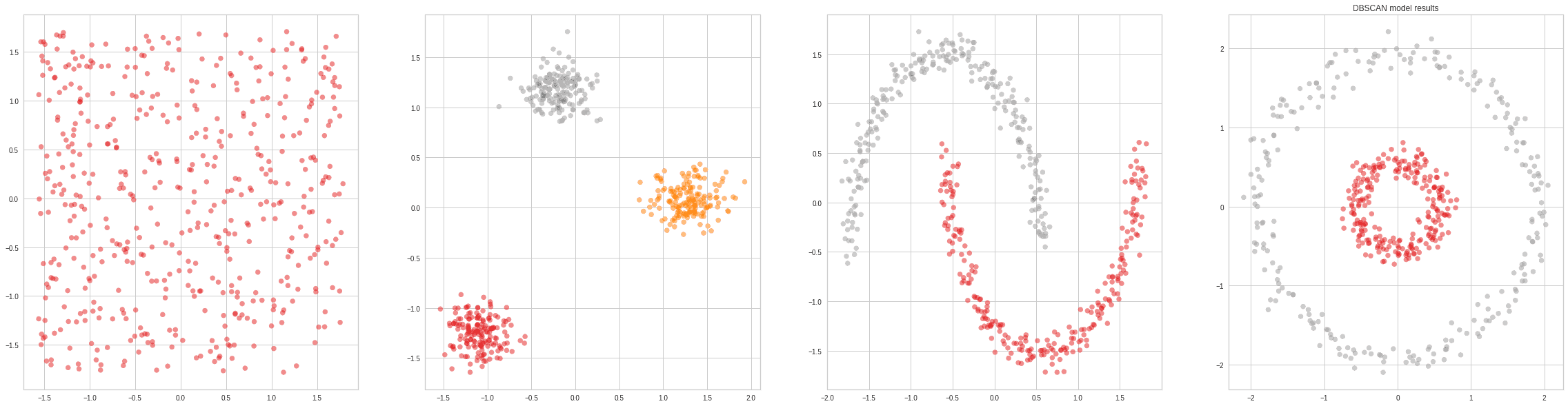
For reference, here’s the result of applying DBSCAN on a couple of toy datasets:
4.1. K-Means Clustering
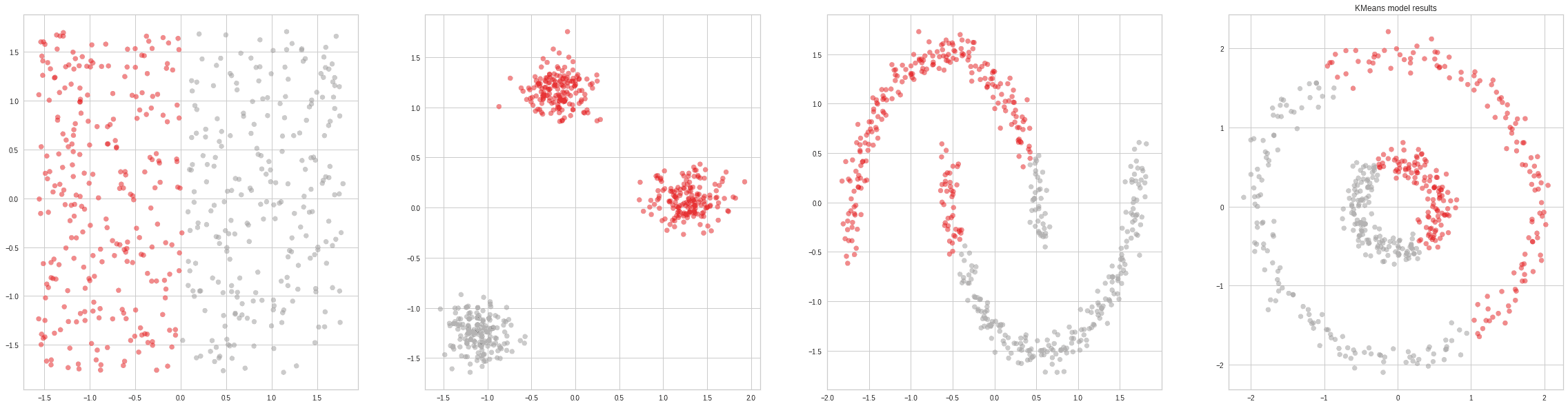
Typically, the most popular clustering algorithm in introductory courses as it is easy to explain, understand and visualize. K-Means Clustering is an algorithm that takes one hyperparameter (the number of clusters) and generates the centroids of those clusters.
Naturally, knowing the true number of clusters beforehand rarely happens. There are some methods to automatically determine the probable number of clusters (the elbow method). Still, in general, they are not so reliable, so K-Means will often under or over-estimate this amount.
Another big drawback of the algorithm is that it only works on convex clusters (clusters that look like blobs with little overlap and no holes). This is extremely limiting, even in the 2D case:
4.2. HDBSCAN
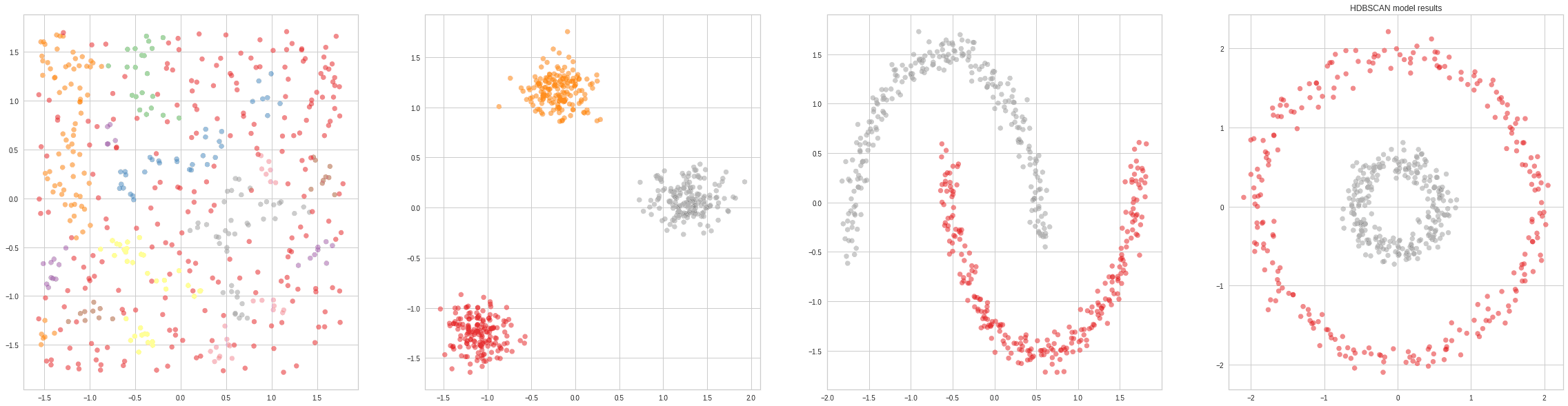
An improvement over DBSCAN, as it includes a hierarchical component to merge too small clusters. Hierarchical DBSCAN is a more recent algorithm that essentially replaces the epsilon hyperparameter of DBSCAN with a more intuitive one called min_cluster_size.
Depending on the choice of min_cluster_size, the size of the smallest cluster will change. Choosing a small value for this parameter will lead to a large number of smaller clusters, whereas choosing a large value will lead to a small number of big clusters.
The greatest drawback of HDBSCAN compared to regular DBSCAN is the fact that it’s not as easy to parallelize. So, if the input has 100s of GB of data, which would require distributing computation among computers in a cluster, DBSCAN would be the best available choice:
5. Conclusion
In this article, we talked about DBSCAN, a really popular clustering algorithm. We first gave some background on the topic of clustering as a whole, then gave a classification of clustering algorithms. Next, we defined the key terms of DBSCAN, gave some intuition for its general functioning and explained it in a step-by-step way. Finally, we compared its performance with 2 other well-known algorithms: K-Means Clustering and HDBSCAN.