How to Calculate the Number of Different Binary and Binary Search Trees

1. Overview

In this tutorial, we’ll learn about the way of computing the number of different Binary and Binary Search Trees (BSTs). Also, we’ll introduce an intuitive explanation of these formulas. We assume having a basic knowledge of Binary Tree and BST data structures.

2. Binary and Binary Search Trees

As we know, the BST is an ordered data structure that allows no duplicate values. However, Binary Tree allows values to be repeated twice or more. Furthermore, Binary Tree is unordered. These are the key differences between those two data structures.

The BST allows traversing its values in sorted order. Balanced BSTs guarantee all the operations on the trees to have $O(log(n))$ time complexity. That is why they are applied in various fields of programming. For instance, Red-Black Trees are self-balancing Binary Search Trees. These are used as an internal implementation of TreeMap in Java. Binary Trees are rarely used because they don’t expect operations (e.g. search, insert, find) to run efficiently.

3. A Number of Binary Search Trees

Suppose the tree has $n$ nodes. It means it contains $n$ unique numbers as values of its nodes. In this section, we’ll define a simple recursive formula. With it, we’ll find the number of structurally different Binary Search Trees of size $n$ .

3.1. Intuitive Explanation

A tree always has a root. We have $n$ possible ways to choose a root. Important to remember, all elements in a tree are distinct. So, without loss of generality, the elements might be a list of numbers from 1 to $n$ . Actually, in solving this problem, we don’t really care what elements we have. The main idea is that they are unique.

If we choose the smallest element as the root of the tree, then we can insert zero values on its left subtree. But if we do, such insertion will violate the main BST property: all values in the left subtree must be less than the root and vice versa for the right subtree. However, we can insert the rest $\boldsymbol{n - 1}$ values in the right subtree.

Generalizing, for node $\boldsymbol{k, k < n}$ , we can insert $\boldsymbol{k - 1}$ nodes to the left subtree and $\boldsymbol{n - k}$ nodes to the right subtree. Moreover, we can do it for each $k$ from 1 to $n$ .

Now, if the root is fixed, the total number of ways to build different trees will be $N_{left} \times N_{right}$ . $N_{left}$ is number of different left subtrees and $N_{right}$ is number of different right subtrees. Let’s move forward with the recursive formulas.

3.2. Recursive Approach

Using the above statements, we can construct a recursive formula $F$ . Let $\boldsymbol{F(n)}$ be the number of different Binary Search Trees of $\boldsymbol{n}$ nodes. Notice, the number of different trees of a tree, which contains a single node is 1. So, $F(1)$ is 1. Similarly, if the tree is empty, then there is 1 possible tree (only this empty one), and $F(0) = 1$ . For any other case starting from 2:

$F(n) = F(0) * F(n - 1) + F(1) * F(n - 2) + \ldots + F(n - 1) * F(0) =$ $\displaystyle \sum_{k=0}^{n - 1} F(k) * F(n - k - 1)$ .

Let’s look at an example of building all possible Binary Search Trees of 1, 2, and 3 nodes respectively:

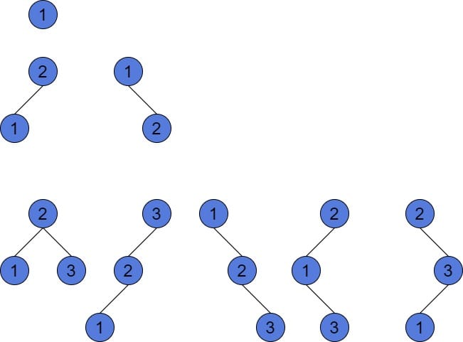
As we may notice, there are only 5 possible BSTs of 3 nodes. But, there exist more than 5 different Binary Trees of 3 nodes. We’ll pay attention to it in Section 5.

4. Catalan Number

Finally, we’re very close to introducing the fact that the number of different BSTs is a Catalan number. This number is often used in different combinatorial problems, like polygon triangulation or valid brackets sequences. The Catalan number sometimes can describe the number of objects, which are defined recursively. In our case, the Catalan number is $\boldsymbol{F(n)}$ .

So, the introduced recursive formula $F$ is $F(n) = Catalan_{n} = (2n)! / ((n + 1)! * n!) = 1 / (n + 1) {2n \choose n}$ . The proof is not trivial and is out of the scope of this article.

5. Number of Binary Trees

Let’s now assume we have only distinct values in our Binary Tree. Unlike the Binary Search Tree, our tree doesn’t have any rules, which we have to follow. So, what does it mean for us? It means, that for every different structure of a Binary Tree, we can also rearrange its node values to get other trees. For better understanding let’s look at the picture:

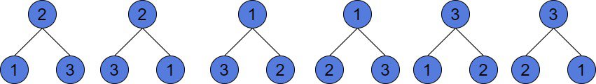
These trees are all structurally equal to each other. The structure of nodes is the same: the tree has just a root and both children. However, we can rearrange the node values in $6 = 3!$ different ways. To do it, we can follow a simple algorithm.

Let’s suppose we have a tree of $n$ nodes. Firstly, we choose an arbitrary node and assign any of $n$ values. Secondly, we choose the next node. To assign the next value to it, we are to choose between $n - 1$ values left. Finally, for the last node, we would have no choice of value, because only one value will be left.

As a result, our simple algorithm explains that for $n$ nodes and the fixed structure of a tree there might be $n!$ different trees.

Summarizing, the number of different Binary Trees is $\boldsymbol{n! / (n + 1) {2n \choose n}}$ . However, this is true only if all elements are distinct. If they are not, then the numerator will look a bit different.

5.1. Permutations with Repetitions

$P_{n} = n!$ is a special case of a formula for permutations because there are no repetitions. We’ll expand it a bit.

We can collect all values to a set of $n$ numbers $(a_{1}, a_{2}, ... , a_{m})$ , where $m < n$ , if they are not distinct. And $m = n$ if they are. Let $k_{1}, k_{2}, ..., k_{m}$ be a count of their repetitions. Notice, $\displaystyle \sum_{i=1}^{m} k_{i} = n$ Then the formula of permutations with repetitions will be:

$P_{k_{1}, k_{2}, \ldots , k_{m}} = \displaystyle \sum_{i=1}^{m} k_{i} / (k_{1}! * k_{2}! * \ldots * k_{m}!) = n! / (k_{1}! * k_{2}! * \ldots * k_{m}!)$ .

If $m = n$ , then $k_{i} = 1$ , $\forall i \in {1 \ldots n}$ . And $P_{k_{1}, k_{2}, \ldots , k_{m}} = P_{n} = n!$ .

5.2. Number of Different and Structurally Different Binary Trees

As a result, the final formula for the number of Binary Trees of $\boldsymbol{n}$ nodes is $\boldsymbol{P_{k_{1}, k_{2}, \ldots , k_{m}} / (n + 1) {2n \choose n}}$ . $k_{1}, k_{2}, \ldots , k_{m}$ are the repetitions of $(a_{1}, a_{2}, ... , a_{m})$ values of the tree, where $m \leq n$ . This is a general formula, which can be used for the trees with unique and not unique values.

However, the number of structurally different Binary Trees is equal to the number of different Binary Search Trees. The number of different BSTs is the Catalan number.

6. Conclusion

In this article, we’ve learned the way to calculate the number of different Binary and Binary Search Trees. Moreover, we’ve revised some formulas from combinatorics. Furthermore, we’ve introduced an intuitive explanation of the calculation formulas. As we can see, the structure of a tree sometimes does matter, however, the values are not. These are the key points for choosing the proper formula.

Full Archive

About Baeldung

Core Concepts

Operating Systems

Artificial Intelligence

Graph Theory

Latex