

Learn through the super-clean Baeldung Pro experience:
>> Membership and Baeldung Pro.
No ads, dark-mode and 6 months free of IntelliJ Idea Ultimate to start with.
Learn through the super-clean Baeldung Pro experience:
>> Membership and Baeldung Pro.
No ads, dark-mode and 6 months free of IntelliJ Idea Ultimate to start with.
Because of their simplicity and versatility, we use metaheuristic algorithms to solve a wide range of engineering and scientific challenges. In particular, they have emerged as effective methods for solving NP problems exactly or approximately.
In this tutorial, we’ll go over a recently proposed metaheuristic algorithm: Black Widow Optimization (BWO).
The inspiration for the BWO algorithm came from the mating process of black widow spiders.
Firstly, the black widow spider cannibalizes its mate after mating. Secondly, the spider displays aggressive behavior to capture prey. Furthermore, the spider builds its agents in a specific pattern to maximize its chances of catching prey.
The algorithm mirrors those behavioral patterns by destroying weak spiders (solutions) and guiding the population of artificial agents to the optimal solution following an artificial spider agent.
In this section, we will go deeper into the mechanism of BWO.
Here is the flowchart of the algorithm:
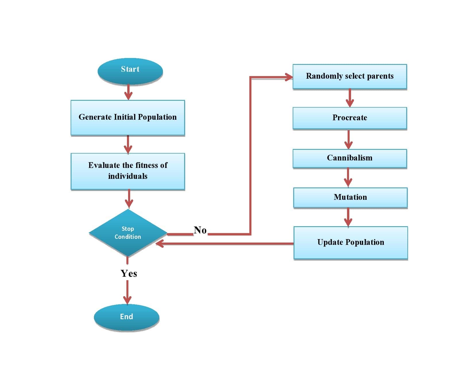
BWO starts by randomly initializing the population of agents referred to as the widows. Using a specially designed score, these agents are then evaluated based on their fitness for the problem at hand.
Subsequently, the algorithm pairs up the best agents and eliminates the weakest through a process of mating and cannibalism. The position of these agents in the solution space is then used to construct a web that facilitates the search for the best solution.
As the algorithm progresses, the group of agents (population) is continuously updated to improve its overall fitness. The process continues until a satisfactory solution, or a predetermined stopping point is reached. This means that the solutions gradually become better and better (based on the fitness value returned from the objective/fitness function), aiming to find a single global optimal solution (the best solution compared to all others in the population).
The combination of mating, cannibalism, and web building helps the Black Widow Optimization algorithm to navigate complex optimization problems and find optimal solutions efficiently.
Here’s the pseudocode:
algorithm BlackWidowOptimization(N, D, ReproductionRate, CannibalismRate, MutationRate, f):
    // INPUT
    //    N = the population size
    //    D = the problem dimensionality
    //    ReproductionRate = the rate of reproduction
    //    CannibalismRate = the rate of cannibalism
    //    MutationRate = the rate of mutation
    //    f = the fitness function
    // OUTPUT
    //    the best found solution

    Initialize widows, the random initial population of widows

    Evaluate each widow from widows

    best <- find the best widow

    // How many widows to mate
    N_R <- N * ReproductionRate

    // Start the main loop
    while stop condition not met:
        // The procreation phase
        parents <- the N_R best widows from widows
        children <- an empty array
        best <- find the best widow from widows

        for i <- 1 to N_R:
            Randomly select two solutions from parents
            Generate D children
            Remove the father spider from parents
            Include the best CannibalismRate * D children into array children

        // The mutation phase
        mutated <- an empty set

        for i <- 1 to N * MutationRate:
            Randomly select a child from children
            Mutate it
            Include it into mutated

        widows <- append children and mutated

    return best
First, we set the algorithm’s parameters: the number of widows and the reproduction, cannibalism, and mutation rates. Additionally, we define a fitness function to evaluate the widows, i.e., candidate solutions.
The algorithm starts by randomly initializing the population of widows. Then, it iteratively applies the procreation (reproduction), cannibalism, and mutation steps.
In the procreation phase, we randomly select widows for mating. As a result, we get their offspring, a set of solutions derived from the parents.
Let  be the problem’s dimensionality and
  and
and  be two individuals (-dimensional vectors) selected for mating. We get children by running the following two steps
  times:
[details]
![\[\left\{\begin{array}{l} y_1=\alpha \times w'+(1-\alpha) \times w'' \\ y_2=\alpha \times w'' +(1-\alpha) \times w' \end{array}\]](/wp-content/ql-cache/quicklatex.com-baa2a79cf434fa4c4769dbbdc6a94286_l3.svg "Rendered by QuickLaTeX.com")
Here,  is a -dimensional array of random numbers from
 ![[0, 1]](/wp-content/ql-cache/quicklatex.com-944fdd98d4f1854c8720f98d8b20b6ad_l3.svg "Rendered by QuickLaTeX.com") , and
, and  and
and  represent the offspring.
Cannibalism is when spiders eat members of the same species. In nature, there are three scenarios of cannibalism: when a female eats its mate, when babies eat their mother, or when a strong baby eats its sibling.
BWO algorithm does cannibalism in two ways.
First, it destroys the father after each mating. When two widows mate, the father is the solution with a worse fitness value.
Another type of cannibalism is called sibling cannibalism. We implement it by keeping several top solutions we get as children in the reproduction step.
In the mutation phase, we select a random number of individuals from the children population. Each of the chosen solutions randomly exchanges its two elements.
After applying mutation, we replace the old population of spiders with the.
The algorithm goes on until meeting the stopping criteria. For example, until reaching the maximum number of iterations.
To keep the population size constant at  throughout the algorithm, the number of children that survive an iteration must be equal to the number of widows removed from the population.
Thus, the number of parents selected for procreation is  , half of which are fathers, so the number of spiders removed in an iteration is
  . The total number of children that survive an iteration is:
![\[\underbrace{N \times ReproductionRate \times D}_{\text{reproduction}} \underbrace{\times CannibalismRate}_{\text{cannibalism}} \underbrace{\times (1 + MutationRate)}_{\text{mutation}}\]](/wp-content/ql-cache/quicklatex.com-3a959970dce6445eb4a132bc264975c4_l3.svg "Rendered by QuickLaTeX.com")
To maintain a population size of  , that number should be equal to , i.e.:
![\[\begin{aligned} &N \times ReproductionRate \times D \times CannibalismRate \times (1 + MutationRate) = N \times ReproductionRate / 2 \\ &D \times CannibalismRate \times (1 + MutationRate) = \frac{1}{2} \end{aligned}\]](/wp-content/ql-cache/quicklatex.com-eac3b58bf1b6104aacd1056eda155146_l3.svg "Rendered by QuickLaTeX.com")
In this article, we talked about the Black Widow Optimization algorithm (BWO). The inspiration for the BWO came from the unique mating behavior of the black widow spiders in nature.
The Black Widow Optimization algorithm has been tested on different problems and works well in terms of finding solutions quickly and accurately. It has also been compared to other popular optimization algorithms and does just as well as them.