

Yes, we're now running our only Summer Sale. All Courses are 30% off until 20th July, 2026:
Learn through the super-clean Baeldung Pro experience:
>> Membership and Baeldung Pro.
No ads, dark-mode and 6 months free of IntelliJ Idea Ultimate to start with.
1. Overview
In this tutorial, we’ll talk about the binary search tree (BST) data structure focusing more on the case where the keys in the nodes are represented by strings.
2. Introduction
A BST is a binary tree that satisfies the following properties for every node:
- The left subtree of the node contains only nodes with keys lesser than the node’s key
- The right subtree of the node contains only nodes with keys greater than the node’s key
- The left and right subtree each must also be a binary search tree.
In this article, we focus more on the case where the keys of the nodes are represented by strings and not numbers. In this case, we should first define the ordering of the strings.
Lexicographic ordering is defined as the order that each string that appears in a dictionary. To determine which string is lexicographically larger we compare the corresponding characters of the two strings from left to right. The first character where the two strings differ determines which string comes first. Characters are compared using the Unicode character set and all uppercase letters come before lowercase letters.
For example:
- apple < orange because ‘a’ comes before ‘o’
- Orange > orange because ‘O’ comes after ‘o’
- apple = apple because all letters are the same
Let’s take a look at two binary trees with strings:
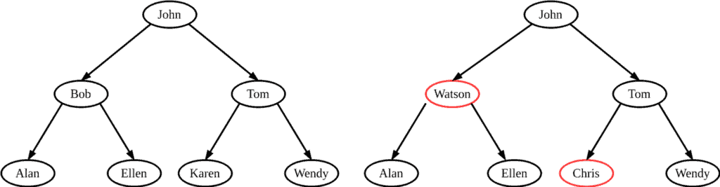
The left tree is a BST since it satisfies the above criterion while the right tree is not a BST because in the red nodes the criterion fails. ‘Watson’ is lexicographically larger than ‘John’ and ‘Chris’ is lexicographically smaller than ‘John’.
3. Basic Operations
As the name suggests, the most frequent operation in a BST with strings is searching for a specific string. Starting from the root we follow a downward path until we find the requested string.
For each node we encounter, we lexicographically compare the requested string  with the node’s string
  . If
. If  , we continue the search in the left subtree since the BST property implies that could not be stored in the right subtree. Symmetrically, if
  we search the right subtree. The whole procedure is summarized in the above pseudocode:
algorithm BSTSearch(node, S):
    // INPUT
    //    node = the current node in the BST
    //    S = the query string to search for
    // OUTPUT
    //    Node if S is found, otherwise a message indicating S is not found

    if node is null:
        return "S not found"
    if S = node.key:
        return node
    if S < node.key:
        return BSTSearch(node.left, S)
    return BSTSearch(node.right, S)
Other useful operations are to insert or delete a specific string from the BST. The data structure must be modified to reflect this change, but in such a way that the binary-search-tree property continues to hold. When inserting a new string, we basically search for the string in the tree using the BST-Search method. When we reach the NULL pointer (since the string is not present in the tree), we insert a node that contains the input string:
algorithm BSTInsert(T, z):
    // INPUT
    //    T = the BST into which z should be inserted
    //    z = the node to insert
    // OUTPUT
    //    BST T with z inserted

    y <- null
    x <- T.root
    while x is not null:
        y <- x
        if z.key < x.key:
            x <- x.left
        else:
            x <- x.right

    z.parent <- y
    if y is null:
        T.root <- z
    else if z.key < y.key:
        y.left <- z
    else:
        y.right <- z
The process of deletion is slightly more intricate. There are three cases:
- If the node has no children, we simply remove it
- If the node has just one child, we replace the node with its child
- If the node has two children, we find its successor that lies in the right subtree and has no left child. Then, we replace the node with its successor
Let’s see the pseudocode:
algorithm BSTDelete(T, z):
    // INPUT
    //    T = the BST from which z should be deleted
    //    z = the node to delete
    // OUTPUT
    //    BST T with z deleted

    if z.left is null:
        TRANSPLANT(T, z, z.right)
    else if z.right is null:
        TRANSPLANT(T, z, z.left)
    else:
        y <- TREE-MINIMUM(z.right)
        if y.parent != z:
            TRANSPLANT(T, y, y.right)
            y.right <- z.right
            y.right.parent <- y
        TRANSPLANT(T, z, y)
        y.left <- z.left
        y.left.parent <- y
In order to move subtrees within the binary search tree, we define a subroutine TRANSPLANT, which replaces one subtree as a child of its parent with another subtree. When TRANSPLANT replaces the subtree rooted at node  with the subtree rooted at node
  , node ’s parent becomes node ‘s parent, and ’s parent ends up having as its appropriate child.
The pseudocode for the TRANSPLANT function is as follows:
algorithm TRANSPLANT(T, a, b):
    // INPUT
    //    T = the BST where the transplanting is to occur
    //    a = the node being replaced
    //    b = the node to replace a
    // OUTPUT
    //    BST T with the subtree rooted at a replaced by the subtree rooted at b

    if a.parent is null:
        T.root <- b
    else if a = a.parent.left:
        a.parent.left <- b
    else:
        a.parent.right <- b

    if b is not null:
        b.parent <- a.parent
4. Complexity Analysis
In a BST searching, insertion and deletion run in time  time where
  is the height of the tree:
| Operation | Time Complexity |
|---|---|
| Search |  |
| Insertion | |
| Deletion | |
5. Conclusion
In this article, we presented the basic operations of a BST that contains strings as keys.