

Yes, we're now running our only Summer Sale. All Courses are 30% off until 20th July, 2026:
Complexity of Inserting N Numbers into a Binary Search Tree
Last updated: March 18, 2024
Learn through the super-clean Baeldung Pro experience:
>> Membership and Baeldung Pro.
No ads, dark-mode and 6 months free of IntelliJ Idea Ultimate to start with.
1. Overview
In this tutorial, we’ll discuss the process of insertion in a binary search tree. We’ll demonstrate the insertion process with an example and analyze the complexity of the insertion algorithm.
2. A Quick Recap on Binary Search Tree
A binary search tree (BST) is a tree-based ordered data structure that satisfies binary search property. Binary search property states that all the left nodes in a binary search tree have less value than its root node, and all the right nodes in a binary search tree have greater value than its root node.
A binary search tree is a very efficient data structure for inserting, removing, lookup, and deleting nodes in the tree.
3. Insertion Example
In the insertion process, given a new node, we’ll insert the node in the appropriate position in the BST. The main point here is to find the correct place in BST in order to insert the new node. Also, we need to ensure after the insertion of the new node that the tree satisfies the binary search property.
Let’s take a binary search tree, and we want to insert a node with value  :
:
The pseudocode of the insertion process can be found in a quick guide to binary search trees.
4. Time Complexity of Insertion
4.1. The Worst Case
Let’s assume the existing binary search tree has one node in each level, and it is either a left-skewed or right-skewed tree – meaning that all the nodes have children on one side or no children at all. We want to insert a node whose value is greater than the highest level node’s value in the case of a right-skewed binary search tree or is less than the highest level node’s value in the case of a left-skewed binary search tree. Let’s look at an example to demonstrate these cases:
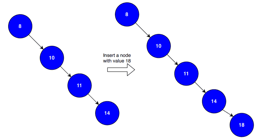
In this example, we’re taking a right-skewed binary search tree, and we want to insert a node with the value  . Notice that the value of the new node is greater than the value of the highest level node in the existing binary search tree.
When we insert a new node, we first check the value of the root node. If the value of the new node is greater than the root node, we search the right subtree for the possible insertion position. Otherwise, we explore the left subtree for the insertion.
The new node here searches the possible insertion position in the right subtree. We compare the value of the new node with all the nodes of the current tree and finds its insertion position at the last level of the binary search tree. Interestingly, in this case, we need to compare the new node’s value with all the nodes in the existing tree. Let’s take an example of a left-skewed binary search tree:
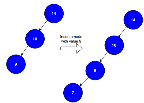
Here, we want to insert a node with a value of  . First, we see the value of the root node. As the new node’s value is less than the root node’s value, we search the left subtree for the insertion. Again we compare the value of the new node with the value of each node in the existing tree. Finally, we insert the new node at the last level of the binary search tree.
In both cases, we have to travel from the root to the deepest leaf node in order to find an index to insert the new node. If there are  nodes in the binary search tree, we need comparisons to insert our new node. Therefore, in such cases, the overall time complexity of the insertion process would be
  .
.
4.2. The Average Case
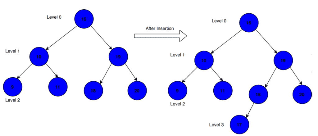
In this case, the existing binary search tree is a balanced tree. Unlike the worst case, we don’t need to compare the new node’s value with every node in the existing tree:
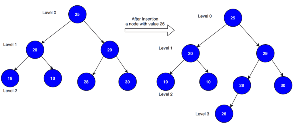
The existing binary search tree is a balanced tree when each level has  nodes, where
  is the level of the tree. Now we want to insert a node with a value
  . First, we check the root node’s value. As it is less than the new node’s value, we explore the right subtree for the insertion. Here the number of comparisons we need to do is
  that’s
  .
.
For any new node that we want to insert, would be the maximum number of comparisons required, which is the height of the binary search tree (Here, L is the level of the existing binary search tree). The height of the binary search tree is also equal to  , where is the total number of the node in the binary search tree.
Therefore in the best and average case, the time complexity of insertion operation in a binary search tree would be  .
.
4.3. The Best Case
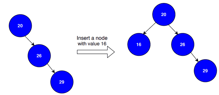
The best-case occurs when all nodes are in the root’s right subtree, the one to be inserted belongs in the left or all nodes are in the root’s left subtree, the one to be inserted belongs in the right. Let’s visualize it with an example:
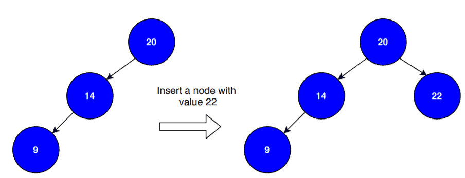
Here the existing binary search tree is a left-skewed tree and we want to insert a new node with the value  that is greater than the root node’s value. As the tree is left-skewed, hence we just need to compare the new node’s value with the root node. Now let’s see another case when the existing tree is right-skewed:
Here the existing tree is a right-skewed tree and the new node’s value is less than the root node. Hence we just need to perform one comparison in order to insert the new node. Therefore in the best case, the time complexity of insertion operation in a binary search tree would be  .
.
5. Conclusion
In this tutorial, we’ve discussed the insertion process of the binary search tree in detail. We presented the time complexity analysis and demonstrated different time complexity cases with examples.