All-Pairs Shortest Paths: Johnson’s Algorithm

1. Introduction

In this tutorial, we’ll discuss Johnson’s algorithm. Along with Floyd-Warshall, it’s one of the algorithms for finding all-pairs shortest paths in directed and undirected graphs. Johnson’s algorithm shows good results for sparse graphs, while Floyd-Warshall is better for dense graphs.

2. Preliminary Notes

For our discussion, we assume we have a graph $G=(V, E)$ . $V$ is the set of vertices of size $N$ , and $E$ is the set of edges of size $M$ . $G$ is a directed graph, and there are no negative-weight cycles in $G$ .

While negative-weight edges are allowed, there must not be negative-weight cycles. The reason is Johnson’s algorithm uses Bellman-Ford and Dijkstra’s single-source shortest paths algorithms (SSSP) as subroutines.

SSSP algorithms don’t work when negative-weight cycles are present. Generally, no shortest paths algorithm makes sense when there’re negative-weight cycles.

3. Algorithm Description

The idea of Johnson’s algorithm is to run Dijkstra’s algorithm for each vertex in $\boldsymbol{G}$ . Unfortunately, that’s workable when there’re no negative-weight edges, as Dijkstra’s algorithm is designed for only non-negative edge weights. To overcome the limitation, the Bellman-Ford algorithm is used to re-weight the edge weights, so there are no negative edge weights.

One can think of an alternative to using the Bellman-Ford algorithm for making the edge weights positive. What if we added the minimum negative edge weight to all the edge weights? That makes the edge weights non-negative, but the idea isn’t workable. If we fix a vertex pair $(u, v)$ , multiple paths may be from $u$ to $v$ . When these paths contain a non-equal count of edges, the path weights get modified differently, so a non-shortest path may become shortest in this way.

Here, we’ll provide a step-by-step explanation of Johnson’s algorithm.

3.1. A New Vertex

We add a new vertex, $s$ , to the graph. Then, we connect $s$ with all the vertices in the graph. The edges are directed from $s$ , and the new edge weights are zero. Thus, $\boldsymbol{s}$ with the new edges doesn’t modify any existing shortest path between the original vertices of the graph.

3.2. Running Bellman-Ford Algorithm

Next, we run the Bellman-Ford SSSP algorithm for $s$ . After this step, we get the shortest paths from $s$ to each graph vertex. Let’s keep the shortest paths in $distance[]$ array, where $distance[v]$ is the shortest path from $s$ to $v$ .

3.3. Re-weighting the Edges

Then, we modify the edge weights. Assume the weight of edge $(u, v)$ is denoted by $weight(u, v)$ , and the new weight of the same edge by $newWeight(u, v)$ . Then, we define the new weights as:

$newWeight(u, v) = weight(u, v) + distance[u] - distance[v]$

The new weights are non-negative because for any edge $(u, v)$ , $distance[v] \le distance[u] + weight(u, v)$ . The inequality follows from the fact that $distance[v]$ is the shortest path from $s$ to $v$ , and if $distance[u] + weight(u, v)$ was less than $distance[v]$ , then there would be a path shorter than the shortest path to $v$ . That contradicts to Bellman-Ford algorithm’s correctness.

Additionally, the weight modification doesn’t change the shortest paths in the original graph. That is, the path weights in the graph actually change, but the shortest paths before and after the weight modification remain the same. Assume we have a path $P$ from vertex $s$ to $t$ , $P = \{(s, v_1), (v_1, v_2), ..., (v_k, t)\}$ . The weight of $P$ before the weight modification is:

$weight(P) = weight(s, v_1) + weight(v_1, v_2) + ... + weight(v_k, t)$

The new weight of $P$ is:

$newWeight(P) = (weight(s, v_1) + distance[s] - distance[v_1]) + (weight(v_1, v_2) + distance[v_1] - distance[v_2]) + ... + (weight(v_k, t) + distance[v_k] - distance[t])) = (weight(s, v_1) + weight(v_1, v_2) + weight(v_k, t)) + (distance[v_1] - distance[v_1]) + (distance[v_2] - distance[v_2]) + ... + (distance[v_k] - distance[v_k]) + (distance[s] - distance[t]) = weight(P) + (distance[s] - distance[t])$

$\boldsymbol{(distance[s] - distance[t])}$ is a constant and doesn’t depend on $\boldsymbol{P}$ , thus if $\boldsymbol{weight(P)}$ was the least before, $\boldsymbol{newWeight(P)}$ would be the least after the weights modification.

3.4. Running Dijkstra’s Algorithm

In the final step, we run Dijkstra’s algorithm for each vertex in the graph with the modified edges. After this step, we’ll have the shortest paths for each vertex pair $(u, v)$ . The shortest path weights are calculated using the modified edge weights.

To calculate the original weights of the shortest paths, we need to parallelly maintain the original weights of the paths during Dijkstra’s algorithm. Alternatively, we can convert the shortest path weights after getting the shortest paths themselves.

4. Johnson’s Algorithm Demonstration on an Example Graph

Let’s pick a directed graph $G$ for our example:

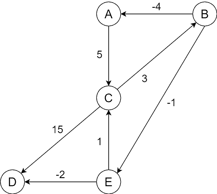
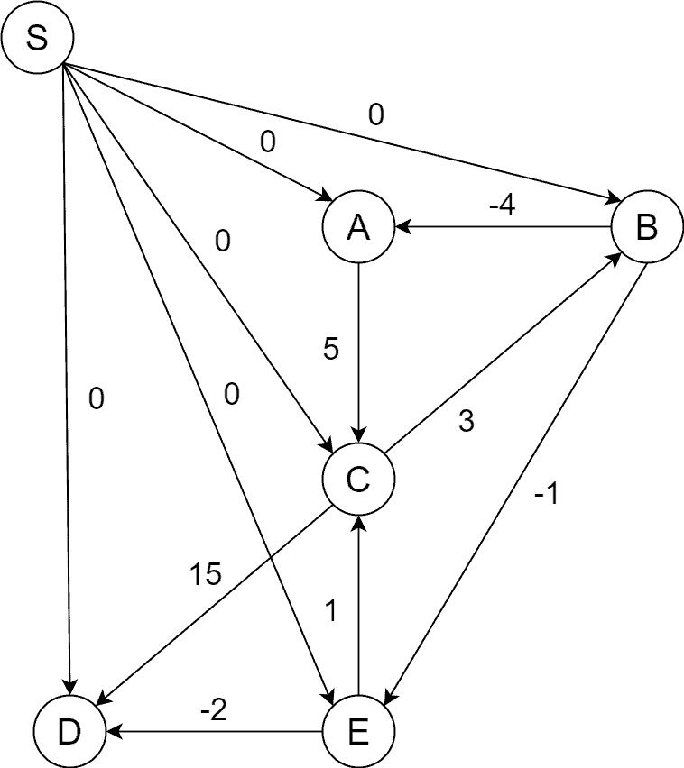
As we can see, there’re negative-weight edges present. Also, there’re cycles in the graph. Nevertheless, there’re no negative-weight cycles. Now, let’s start the algorithm. First, we add a new vertex and introduce the directed zero-weight edges going out of the added vertex. The added vertex is $S$ :

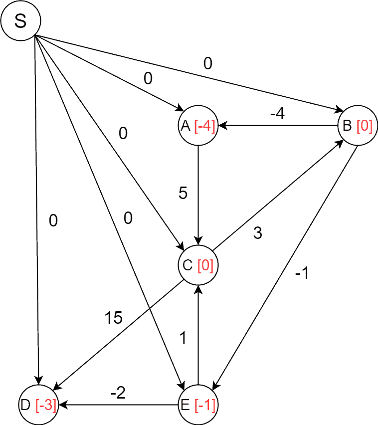
It’s time to run the Bellman-Ford algorithm to calculate the shortest paths from $S$ to all the graph vertices. We can see the shortest paths within the vertex nodes in red. For example, the shortest path’s weight from $S$ to $E$ is $-1$ :

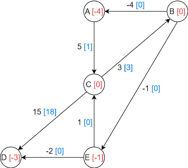
After we’ve calculated the shortest paths from $S$ in the previous step, we can modify the edge weights. The original edge weights are left as is, and the new weights are provided in blue within the brackets:

Finally, the last step is to run Dijkstra’s algorithm on the graph with the modified edge weights. The resulting pair-wise shortest paths matrix is:

We can switch back to the original edge weights. The pair-wise shortest paths matrix will then be:

5. Algorithm Pseudocode

We assume we have functions BELLMANFORD( $G, u$ ) and DIJKSTRA( $G, u$ ) that accept the input graph $G$ and the source vertex $u$ . They return the shortest paths from $u$ to all the remaining vertices in $G$ . The pseudocodes for the algorithms can be found in their appropriate discussions: Bellman-Ford and Dijkstra’s algorithms.

The pseudocode for Johnson’s algorithm will then be:

6. The Complexity Analysis

The time complexity of Johnson’s algorithm depends on Bellman-Ford and Dijkstra’s algorithms. Bellman-Ford algorithm runs in $O(N * M)$ . Each invocation of Dijkstra’s algorithm takes $O(N * log(N))$ time, and we invoke it $N$ times, so the overall complexity of the step is $O(N^2 * log(N))$ .

Thus, Johnson’s algorithm runs in $\boldsymbol{O(N * M + N^2 * log(N))}$ . When $G$ is sparse, this is better than $O(N^3)$ running time of the Floyd-Warshall algorithm. Floyd-Warshall algorithm is preferable when $G$ is a dense graph where almost all vertex pairs are connected.

The space complexity of Johnson’s algorithm is $\boldsymbol{O(N ^2)}$ as it calculates and returns the pair-wise shortest paths matrix.

7. Conclusion

In this topic, we’ve gone over Johnson’s algorithm. It’s an algorithm to find all-pairs shortest paths in directed and undirected graphs. Johnson’s algorithm uses Bellman-Ford and Dijkstra’s single-source shortest paths algorithms as its subroutines. The algorithm is the best for sparse graphs.

Full Archive

About Baeldung

Core Concepts

Operating Systems

Artificial Intelligence

Graph Theory

Latex