Ukkonen’s Suffix Tree Algorithm | Baeldung on Computer Science

1. Introduction

In this topic, we’ll cover Ukkonen’s algorithm. It’s a space-efficient linear-time algorithm for building suffix trees.

2. Recap on Suffix Trees

The suffix tree of a string $\boldsymbol{S}$ is a rooted directed tree built out of the suffixes in $\boldsymbol{S}$ . Each node in the tree is labeled with a substring of $\boldsymbol{S}$ , and no two edges out of the same node start with the same character. Additionally, each suffix ends in a terminal node. To locate a suffix, we need to start from the root node and move along the edges, concatenating their labels in the process until we reach a terminal node.

In our discussion, we assume $S$ is a zero-indexed string. Below is the suffix tree of string $abcd$ :

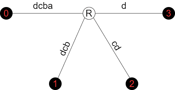
The tree above contains the following suffixes:

$\boldsymbol{d}$ – starts at 3
$\boldsymbol{cd}$ – starts at 2
$\boldsymbol{bcd}$ – starts at 1
$\boldsymbol{abcd}$ – starts at 0

The root node is denoted by $R$ . Each terminal node is black and contains the starting index of the suffix it represents. For example, the terminal node containing 1 represents suffix $bcd$ which starts at position 1 in $abcd$ .

The example above is a primitive suffix tree for a string without repeating characters. Such simple suffix trees don’t contain internal nodes. For complex strings, the suffix tree is complex as well. Below is the suffix tree of string $abcabcde$ :

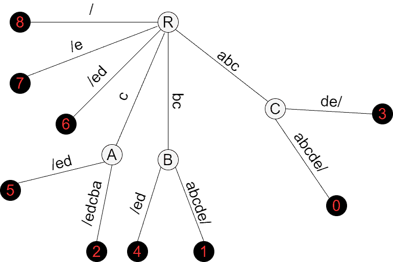
Note that we append the slash symbol at the end of the string. That’s done for the suffixes to end in terminal nodes. Without it, suffixes will end in the middle of edges or in internal nodes. We could actually append any character that is absent in $S$ instead of the slash. The suffix tree represents the following suffixes:

$\boldsymbol{/}$ – starts at 8
$\boldsymbol{e/}$ – starts at 7
$\boldsymbol{de/}$ – starts at 6
$\boldsymbol{cde/}$ – starts at 5
$\boldsymbol{bcde/}$ – starts at 4
$\boldsymbol{abcde/}$ – starts at 3
$\boldsymbol{cabcde/}$ – starts at 2
$\boldsymbol{bcabcde/}$ – starts at 1
$\boldsymbol{abcabcde/}$ – starts at 0

It’s very easy to build the suffix tree for strings with non-repeating characters. In such suffix trees, there’re no internal nodes, and a single edge connects each terminal node to the root. Complications arise when characters repeat, and we need clever algorithms that build suffix trees efficiently.

3. A Straightforward Approach for Building Suffix Trees

An intuitive approach to building the suffix tree of the given string $S$ is to insert each suffix gradually. For example, we can insert the suffixes starting from the shortest suffix and ending with the longest one. We can also insert the suffixes in the opposite order. Or we can even insert them randomly. Anyway, the result is the same suffix tree.

The time complexity of the approaches that directly insert the suffixes in some order is $\boldsymbol{O(N^2)}$ , where $\boldsymbol{N}$ is the length of $\boldsymbol{S}$ : there’re $\boldsymbol{N}$ suffixes, and each one is inserted in $\boldsymbol{O(N)}$ time.

4. Ukkonen’s Algorithm

This section describes Ukkonen’s algorithm for building suffix trees. The algorithm builds a series of implicit suffix trees, one for each prefix of $S$ . The final implicit suffix tree then appears to be the suffix tree of $\boldsymbol{S}$ as the last character of $\boldsymbol{S}$ is distinct.

Let’s denote the substring of $S$ starting at position $i$ and ending at $j$ by $S[i, j]$ . Additionally, let’s denote the implicit suffix tree of prefix $S[0, j]$ by $IST_j$ . So, the algorithm builds $IST_0$ , then $IST_1$ , etc. $IST_{N - 1}$ is built in the end. $IST_j$ is built using $IST_{j - 1}$ , $j > 0$ .

More specifically, here’re the steps of the algorithm:

Build $IST_0$
For j = 1 to $N - 1$ , build $IST_j$ on top of $IST_{j - 1}$

And below are the steps to build $IST_j$ having $IST_{j - 1}$ :

Fix prefix $S[0, j]$
$IST_j = IST_{j - 1}$
For i = 0 to $j$ , add suffix $S[i, j]$ to $IST_j$

As we see, each suffix of $S[0, j]$ is added to $IST_{j - 1}$ to get $IST_j$ .

First, we’ll explore the compound parts of the algorithm. Then, we’ll demonstrate the algorithm with an example.

4.1. Implicit Suffix Trees

An implicit suffix tree is a tree that is built from the suffix tree by removing the slash, then removing edges without labels and their terminal nodes, then removing internal nodes with a single outgoing edge. Thus, the implicit suffix tree is very similar to the suffix tree in that it contains all the suffixes of the original string. The only difference is that not all the suffixes may end in terminal nodes, some of them may end in internal nodes or even in the middle of edges.

When $\boldsymbol{S}$ consists of distinct characters, the implicit suffix tree is the same as the suffix tree. There’s also a weaker condition when the two match: if the last character of $S$ has no other entries in the string. In both cases, no suffix is a prefix of another suffix. Below is the implicit suffix tree of string $abcabc$ :

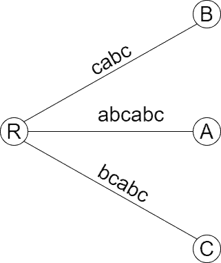
The implicit suffix tree above contains all the suffixes of $abcabc$ :

$\boldsymbol{c}$ – ends in the middle of edge (R, B)
$\boldsymbol{bc}$ – ends in the middle of edge (R, C)
$\boldsymbol{abc}$ – ends in the middle of edge (R, A)
$\boldsymbol{cabc}$ – ends in terminal node B
$\boldsymbol{bcabc}$ – ends in terminal node C
$\boldsymbol{abcabc}$ – ends in terminal node A

Besides, the tree also contains strings that aren’t suffixes of $abcabc$ , e.g., $cab$ .

4.2. Extension Rules

There’re three suffix extension rules used by the algorithm to get $\boldsymbol{IST_{j}}$ from $\boldsymbol{IST_{j - 1}}$ , $\boldsymbol{j > 0}$ :

Rule 1 – All the existing suffixes ending in terminal nodes of $IST_{j - 1}$ get extended by $S[j]$ . No additional work is done for such suffixes.
Rule 2 – Suffix $S[i, j]$ doesn’t have continuation starting at position $k, i \le k \le j$ when tracking its path down the root. In this case, we need to add a new terminal node, along with a new edge with the label $S[k, j]$ leading to it. If label $S[i, k - 1]$ ends in an internal node, then no new internal node is added, otherwise, we add an internal node. If $S[i, k - 1]$ ends in the middle of an edge, the edge is split into two parts, an internal node is added between the parts and an outgoing edge with label $S[k, j]$ is added to the new internal node.
Rule 3 – When suffix $S[i, j]$ ends in an internal node or in the middle of an edge, do nothing and go to the next phase.

5. Optimizations

If we simply follow the steps of the algorithm, we get an $\boldsymbol{O(N^3)}$ algorithm for building suffix trees. It’s worse than the straightforward approach discussed earlier. The asymptotic is obvious, as there’re $N$ implicit suffix trees to be built, and each one is built using $O(N^2)$ time by inserting O(N) suffixes of the current prefix in O(N) time each.

We leverage several optimizations to turn the algorithm into a linear one:

5.1. Edge Label Compression

This optimization helps to reduce space usage. Instead of keeping the actual substrings for edge labels, we keep the coordinates of substrings in $S$ , i.e. the substrings’ start and end indices in $S$ .

5.2. Global End

We can observe that once a suffix is added to an implicit suffix tree, i.e., when it ends in a terminal node, it can be extended automatically by appending the current extension symbol to it. More specifically, we apply Rule 1 for such suffixes by keeping the global end index. The global end is written as the ending index of the edges leading to terminal nodes.

5.3. Termination for the Current Phase

If some substring $S[i, j]$ is present in the current implicit suffix tree, then all the suffixes of $S[i, j]$ must also be present by the definition of the algorithm. Thus, once we observe it, we stop building $IST_j$ and move to $IST_{j + 1}$ .

5.4. Suffix Links

Suffix links are used to add suffixes that only differ in some starting symbols quickly. For example, if suffix $S[i, j]$ is present in the current implicit suffix tree and we’re adding suffix $S[i, j + 1]$ , then the rest of the remaining suffixes $S[i + 1, j + 1]$ , $S[i + 2, j + 1]$ and etc., are added efficiently by using the previously gathered information.

Suffix links enable jumps between the internal nodes and the root. Suffix links point from internal nodes to other internal nodes or to the root node. They are created during the algorithm.

5.5. Skip/Count

To move fast in the tree, we keep the lengths of the edges. Along with the active state variables described in the following example, this trick enables us to locate suffixes very quickly.

6. Demonstration of the Algorithm

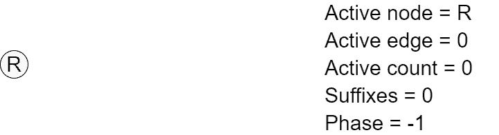
In this section, we’ll build the suffix tree for string $abcabcde$ step by step using Ukkonen’s suffix tree algorithm. During the process, we maintain the variables related to the active state:

Active node – Node in the tree from which the algorithm continues the next step
Active edge – Direction to which move from the active node. As each outgoing edge of a node starts with a distinct symbol, this is simply the index of a symbol in $S$
Active count – Number of symbols to skip when moving from the active node in the active direction
Suffixes – Number of suffixes to build left from the previous steps
Phase – Phase number. The global end is equal to the phase number

Initially, we have the root node:

Then, we add the single suffix of prefix $S[0, 0]$ = $a$ :

Note that we display the edge labels for verbosity, according to the edge label compression, they’re absent, and only the [start, end] index pair is there. The ‘end’ variable is a placeholder for the global end. Next, we consider prefix $S[0, 1]$ = $ab$ :

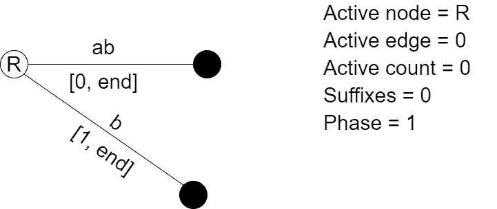
Note how suffix $ab$ got updated automatically, we literally did nothing to update it. We added suffix $b$ using Rule 2 and finished Phase 1. Phase 2 considers prefix $S[0, 2]$ = $abc$ :

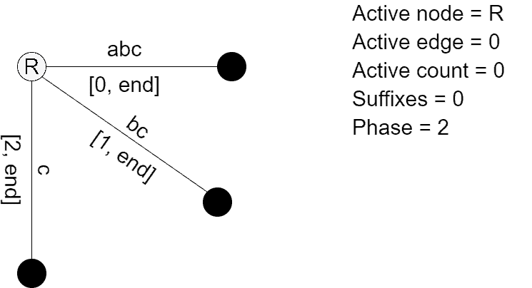
The interesting part starts now. We consider prefix $S[0, 3]$ = $abca$ , and it’s the first case with a repeating character:

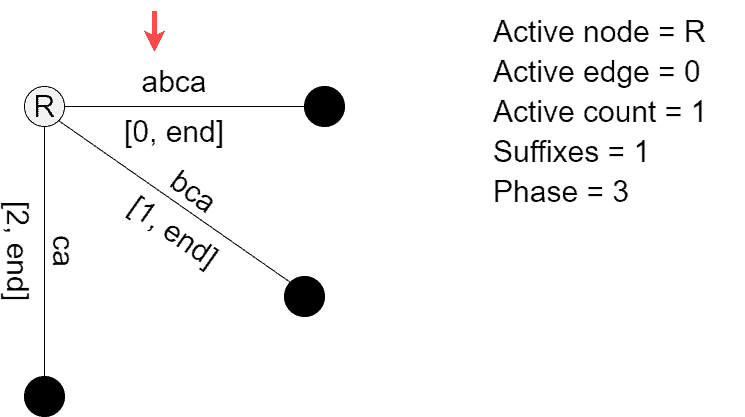
Suffixes $abca$ , $bca$ , and $ca$ got updated automatically according to Rule 1. While trying to insert suffix $a$ , we encountered Rule 3 and terminated Phase 3. The appropriate state variables got updated, and the red arrow now shows the point where the next step starts. Now, prefix $S[0, 4]$ = $abcab$ gets processed:

The suffixes ending in terminal nodes got updated automatically. While comparing $S[4]$ = $b$ to the current symbol located by the state variables, we saw a match; thus, Rule 3 is applied again. We updated the state variables and terminated Phase 4. Phase 5 is similar to Phase 3 and Phase 4:

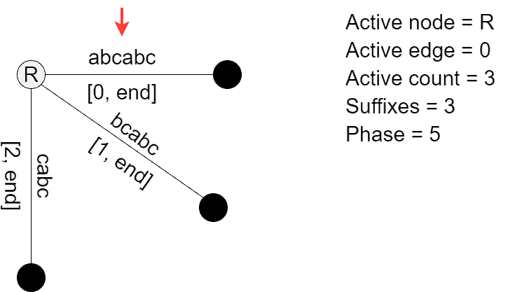
We have accumulated three suffixes to be built in the future steps, namely suffixes $a$ , $ab$ , and $abc$ . Next, we consider prefix $S[0, 6]$ = $abcabcd$ , and it’s the case where $S[6]$ = $d$ and the symbol pointed by the active state differs:

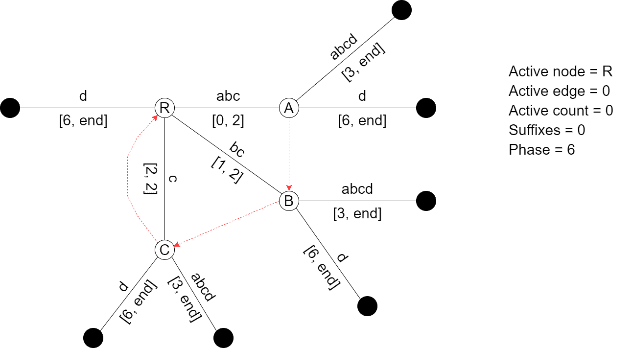
During Phase 6, all the accumulated suffixes were inserted in appropriate places, and suffix links were created. Those suffixes were added according to Rule 2. Additionally, a new branch that represents suffix $d$ was added to the root, and the suffix was added using Rule 2. When we create an internal node, we add a suffix link from it pointing to the root node. Afterward, suppose a new internal node is added during the same phase. In that case, the suffix link of the previously created internal node is redirected from the root to the newly created internal node. This way, all the internal nodes created during the same phase point to each other in the order of their creation, with the last one pointing to the root node.

Note how we updated the active state variables to reflect the changes. Generally, if we jump from an internal node to another internal node using a suffix link, the active node gets the value of the internal node that we jump, and the active edge and the active count remain the same. When we jump from an internal node to the root, the root becomes the active node, the active edge gets incremented, and the active count gets decremented.

After Phase 6, node $A$ points to node $B$ , and node $B$ points to node $C$ . Finally, node $C$ points to the root as it was the last internal node created during Phase 6. In the future, if one of the internal nodes becomes an active node after adding a suffix to its path, we follow its suffix link to insert the same suffix on the path of its suffix link node. The process continues until we encounter Rule 3 or we reach the root node and insert the suffix using one of the three rules.

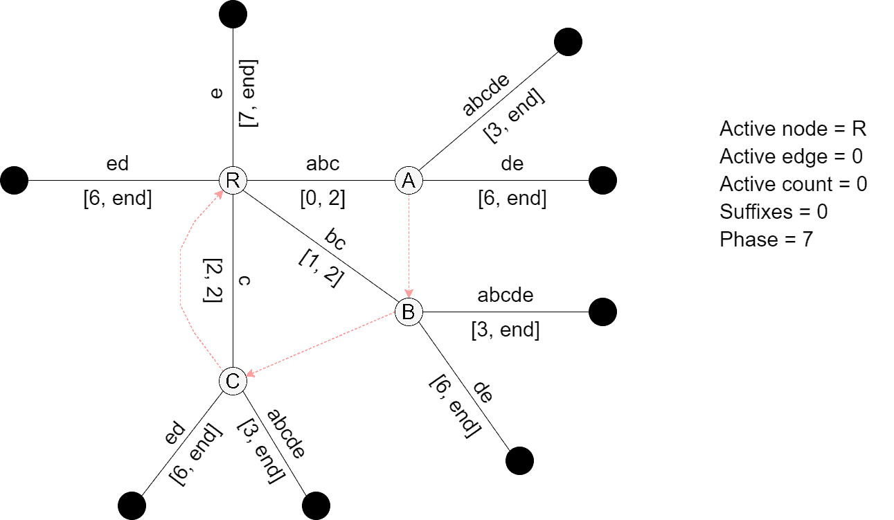
Next, we consider prefix $S[0, 7]$ = $abcabcde$ . The active node is the root, the active count is zero, and symbol $S[7]$ is distinct, so Phase 7 extends the existing suffixes using Rule 1 and adds suffix $e$ using Rule 2:

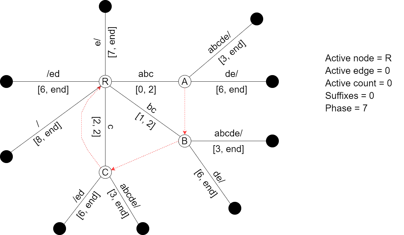
Finally, we add the terminating slash to the tree:

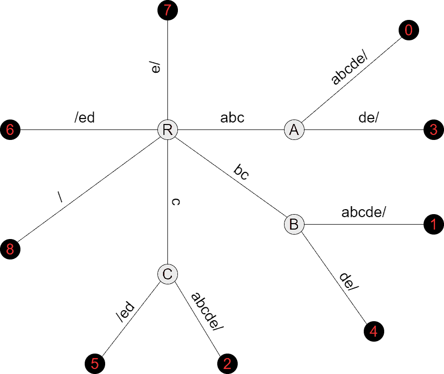
The last step is to traverse the suffix tree using DFS and write the suffix indices in the terminal nodes. We also remove the data used in the suffix tree construction but not used afterward:

The algorithm runs in linear time. The intuition behind that is the algorithm addresses each suffix once in some phase, after which the suffix is extended automatically using Rule 1. Switches between nodes to construct accumulated suffixes take constant time due to all the optimizations discussed previously. For detailed proof of the time complexity, please see Chapter 6 of Algorithms on Strings, Trees, and Sequences, by Dan Gusfield.

7. Conclusion

In this topic, we’ve discussed Ukkonen’s algorithm for building suffix trees in linear time. We started with a short introduction to suffix trees, then we discussed a straightforward approach to building suffix trees. Next, we’ve described Ukkonen’s algorithm and its compound parts. Finally, we’ve demonstrated the algorithm with a step-by-step example.

Full Archive

About Baeldung

Core Concepts

Operating Systems

Artificial Intelligence

Graph Theory

Latex