Learn through the super-clean Baeldung Pro experience:
>> Membership and Baeldung Pro.
No ads, dark-mode and 6 months free of IntelliJ Idea Ultimate to start with.
Last updated: June 11, 2023

Learn through the super-clean Baeldung Pro experience:
>> Membership and Baeldung Pro.
No ads, dark-mode and 6 months free of IntelliJ Idea Ultimate to start with.
In this tutorial, we’re going to explore the differences and nuances of transfer learning and domain adaptation. Transfer learning is a broad term that describes using the knowledge gained from one machine learning problem in another one. Domain adaptation describes a special case of transfer learning that only covers the change of the data domain.
To clarify transfer learning, we compare it to a classical supervised machine learning problem. For a better understanding, we work with a sample dataset of dog and cat pictures.
In a classical setting, we have a dataset  form which we extract our features
  . For those features, we want labels
  , for example, a picture that has the high-level features, foot of a dog, the face of a dog, and body of the dog, we assign the label dog. Thus we have a function assigning values of our set features to our set labels.
When we use the model in production, we have a different but similar dataset, it still shows dogs and cats. And it still assigns those pictures to the same labels “dog” and “cat”.
In this picture, we can see two datasets and  , which are different but similar:
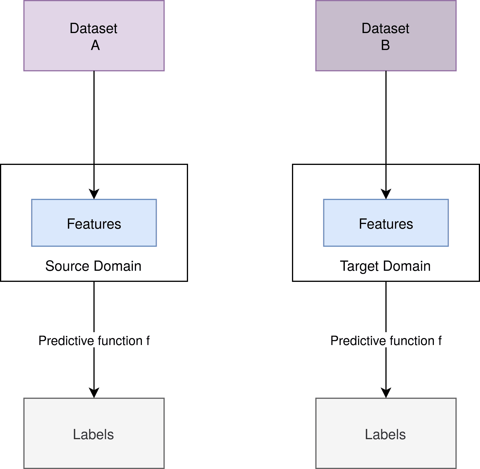
From the datasets, we extract our features. And for a particular set of features, we assign one or more labels. The features, the predictive function  , and the labels remain the same.
Transfer Learning describes a collection of machine learning techniques that work with a structure similar to the classical supervised case. In contrast, it can also work with datasets and features that are vastly different.
Let’s have a look at the structure of a transfer learning process. As we can see, the labels and the predictive function can change:
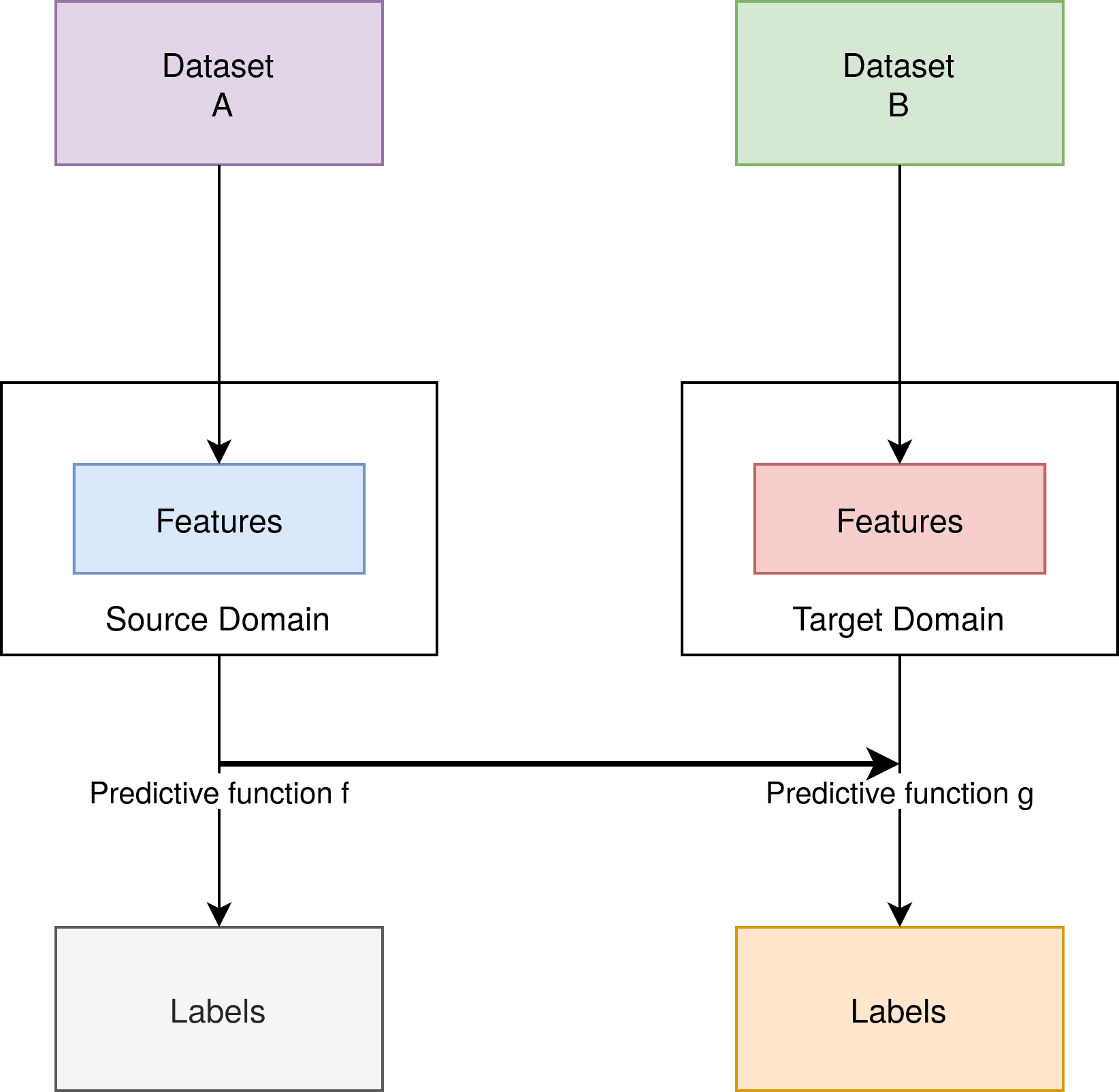
Furthermore, we have a similar structure to supervised learning. But, in heavy contrast, none of the building blocks have to be the same in the case of transfer learning. The connection between the two machine learning settings is the utilization of the predictive function , which is used in the creation of the second predictive function  .
.
It should be noted that in this case, the steps of source and target are different. Transfer learning also includes the other cases, in which e.g. only labels are different and features are the same.
The instance that covers the case of the same labels and vastly different, but similar datasets is a type of transfer learning as well. We will cover this in the section about domain adaptation.
Let’s apply this concept to our example of dog and cat pictures. Now imagine we have a second dataset that shows pictures of cows and horses. Cows and horses are significantly different from cats.
Nevertheless, they are all mammals, they have four feet, and a similar shape. As a solution, we can take the layers that describe the shape of the object we want to detect, whether it is a dog, a cow, or a horse, and freeze them. Freezing means we cut them out of our predictive function put them in our predictive function , and train the function , without training our frozen layers:
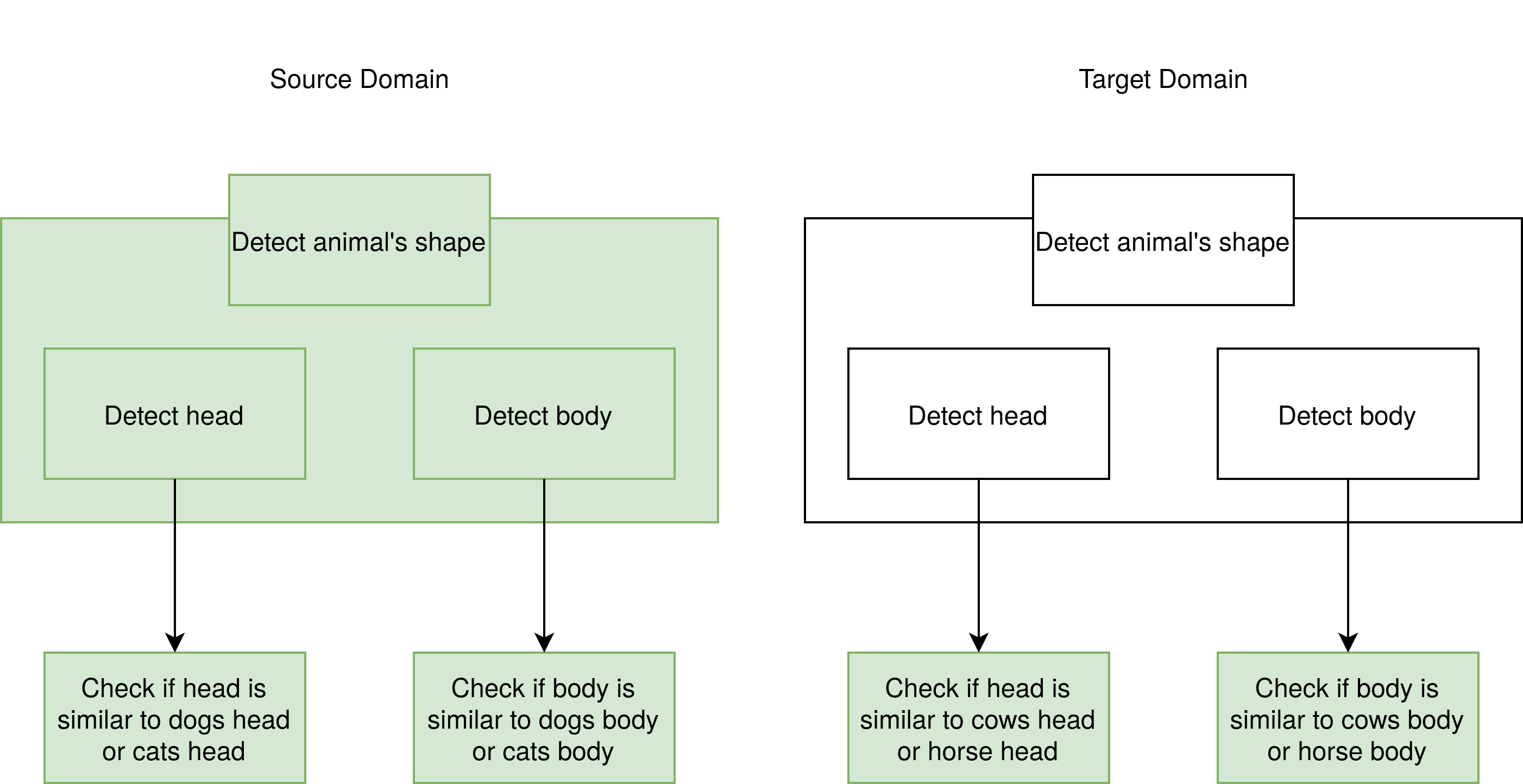
We can see the layers on the right side are green, which indicates that we have to train them while creating our predictive function for the source domain. On the other hand, the predictive is created using the already existing, frozen layer from the source domain. The frozen layers stay untouched during the training process.
Domain adaptation is, as already mentioned, a special case of transfer learning.
In domain adaptation, we solely change the underlying datasets and thus the features of our machine learning model. However, the feature space stays the same. The predictive function stays the same:
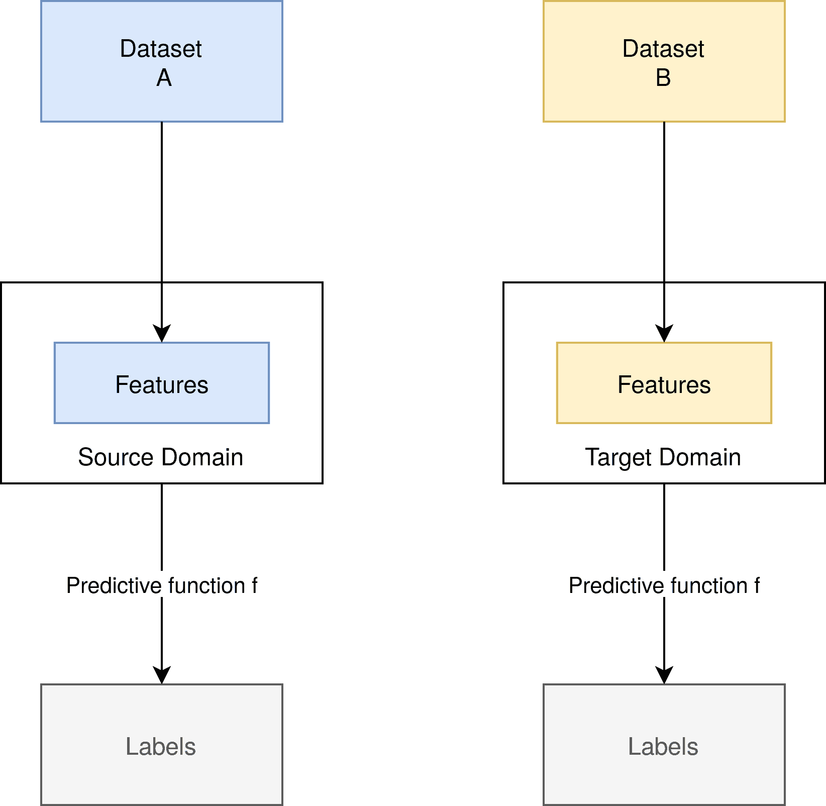
Applying domain adaptation to our example, we could think of a significantly different, but somehow similar dataset. This could still contain dog and cat pictures, but those that are vastly different from the ones in our source dataset. For example, in our source data set, we only have poodles and black cats. In our target dataset, on the other hand, we could have schnauzers and white cats.
Now, how can we ensure that our predictive function will still predict the right labels for our dataset? Domain adaptation delivers an answer for this question.
We consider three types of domain adaptation. These are defined by the number of labeled examples in the underlying domain:
In domain adaptation, we can look a bit closer at pragmatic approaches. This lies in the fact, that only changing the dataset makes it much easier to tune our model for our new machine learning process.
Divergence-based domain adaptation is a method of testing if two samples are from the same distribution. As we have seen in our blueprint illustration, the features that are extracted from the datasets are vastly different. This difference causes our predictive function to not work as intended. If it’s fed by features that it was not trained for, it malfunctions. This is also the reason why we accept different features but require the same feature space.
For this reason, divergence-based domain adaptation creates features that are “equally close” to both datasets. This can be achieved by applying various algorithms, including the Maximum Mean Discrepancy, Correlation Alignment, Contrastive Domain Discrepancy, or the Wasserstein Metric.
In the iterative approach, we use our prediction function to label those samples of our target domain, for which we have very high confidence. Doing so, we retrain our function . Thus creating a prediction function that fits our target domain more and more as we apply it to samples that have less confidence.
As we have seen transfer learning offers a range of methods to use an already existing machine learning model in a new environment. In the special case of domain adaptation, we have an issue frequently encountered in a real-world scenario, a distinct dataset.
For this case the divergence-based domain and domain adaptation and the iterative approach offer solutions. Moreover, these solutions are a big part of contemporary research in the area of machine learning.