How to Draw on an Image with TikZ

1. Introduction

When creating technical documents, diagrams, or presentations in LaTeX, we sometimes need to annotate or draw over existing images. Showing arrows, labels, or shapes over a photograph or a diagram can help us explain concepts more clearly. In LaTeX, we can use TikZ for this task. It’s a versatile drawing library built on top of PGF (Portable Graphics Format) in LaTeX.

In this tutorial, we’ll combine images and TikZ to create annotated graphics. We’ll cover everything from setting up the environment to aligning drawings with the underlying image and provide plenty of examples along the way.

By the end, we’ll understand how to place figures precisely, add labels at exact coordinates, and highlight important regions on an image. This approach can be particularly useful in technical fields like engineering, math, or computer science, where precise labeling or indication of components is crucial.

2. Basic Setup for TikZ

TikZ is included when importing the tikz package in the LaTeX preamble. Here’s a minimal example to get started:

\documentclass{article}
\usepackage{graphicx}  % to include images
\usepackage{tikz}      % TikZ for drawing
\begin{document}

% our content here

\end{document}

Once we do this, we can access the TikZ drawing commands.

Typically, we draw with the tikzpicture environment like this:

\begin{tikzpicture}
  % TikZ commands go here
\end{tikzpicture}

However, to overlay shapes or text on top of an image, we must combine the image and the TikZ commands.

3. Placing an Image in TikZ

One straightforward way to place an image inside a tikzpicture is to use node with the includegraphics command:

\begin{tikzpicture}
  \node[anchor=south west, inner sep=0] (img) at (0,0) {\includegraphics[width=10cm]{example-image.png}};
\end{tikzpicture}

The example image looks like this:

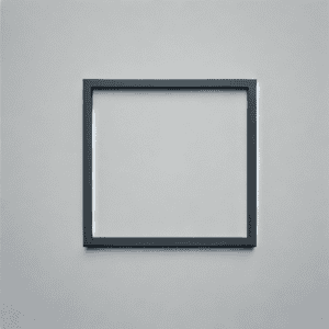
What did we do here?

• We create a node at coordinates (0,0), anchored at south west so that the lower left corner of the image sits at the origin (0, 0) of the TikZ coordinate system.
• We set inner sep=0 to avoid extra padding around the image.
• Finally, we specified the image size using width=10cm.

Now, the entire image is placed in a coordinate plane so that the bottom left corner is at (0,0) and the top right corner is at (10,0). This is because the image is 10cm wide. Additionally, the y-extent depends on the image’s aspect ratio.

4. Annotating the Image

We can overlay shapes, lines, or text with the image established as a node. Let’s place a red circle with a radius of 0.2cm at coordinates (2,3) and label it:

\begin{tikzpicture}
  % Place the image
  \node[anchor=south west, inner sep=0] (img) at (0,0) {
    \includegraphics[width=10cm]{example-image.png}
  };

  % Create a coordinate system matching the image size
  \begin{scope}[x=1cm,y=1cm]
    % Draw a red circle at (2,3)
    \filldraw[red] (2,3) circle (0.2);

    % Label the circle
    \node[above] at (2,3) {Red Circle};
  \end{scope}
\end{tikzpicture}

Here, a few things are happening:

• We use a scope with [x=1cm, y=1cm] to treat each unit in TikZ as 1 cm. This ensures we use the same units (centimeters) as the image we scaled to be 10cm wide.
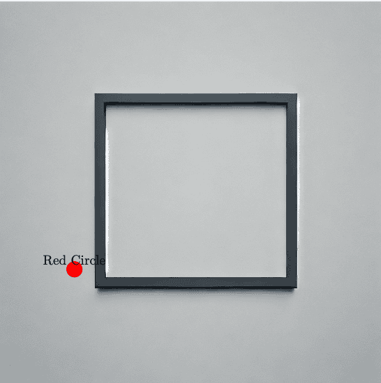
• Then, we place a red filled circle (\filldraw[red]) of radius 0.2 cm at (2, 3).
• Finally, we add a label with the text Red Circle above the circle using \node[above] at (2,3) {Red Circle}.

Upon compiling, we’ll see the image and, on top of it, a small red circle with its label:

5. Overlaying Coordinates with remember picture, overlay

Sometimes, we want to place an image in the normal LaTeX flow (for example, as part of a figure environment) and then want to reference and annotate that same image later in the document.

One approach is to use tikzpicture with overlay and remember picture. This technique is handy if we insert the image via a standard \includegraphics command and then refer to it in a TikZ overlay:

% First, place the image in the document
\begin{figure}[ht]
  \centering
  \includegraphics[width=10cm]{example-image.png}
  \caption{An example image}
  \label{fig:example-image}
\end{figure}

% Now create an overlay referencing the page
\begin{tikzpicture}[remember picture,overlay]
  \node at (current page.center) {
    \begin{tikzpicture}
      % We can place elements relative to current page or find exact offsets
      \draw[red, thick] (0,0) circle (1cm);
    \end{tikzpicture}
  };
\end{tikzpicture}

Here:

• remember picture,overlay instructs TikZ to place these drawing commands over the existing page layout.
• We use references to current page to align shapes exactly over the included image.

Precise alignment requires trial and error or calculating offsets based on known bounding boxes. Here’s the result:

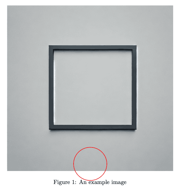
While this method is robust, the more straightforward approach is to embed the image directly inside the tikzpicture environment.

6. Complex Shapes and Paths on the Image

TikZ supports a wide variety of shapes beyond circles and simple labels. We can draw polygons, curves, or even custom shapes to highlight regions of the image. For instance, suppose we want to annotate a rectangular region:

\begin{tikzpicture}
  \node[anchor=south west, inner sep=0] at (0,0) {
    \includegraphics[width=10cm]{example-image.png}
  };

  % Draw a rectangle from (3,2) to (6,4) in blue
  \draw[blue, thick, dashed] (3,2) rectangle (6,4);

  % Put a label near the rectangle
  \node[blue, above] at (4.5,4) {Highlighted Area};
\end{tikzpicture}

Here:

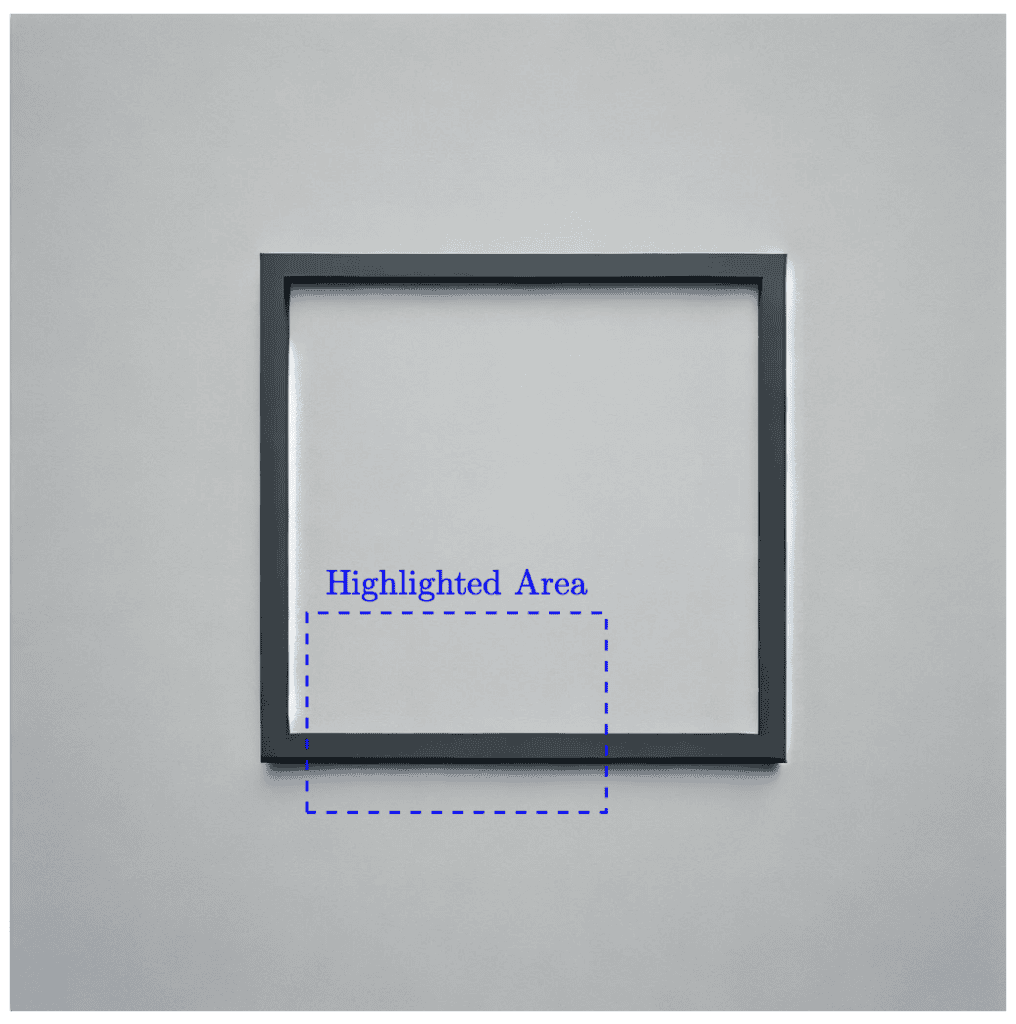
• We define a rectangle with the rectangle path command from (3,2) as the lower left to (6,4) as the upper right corners
• To make it stand out, we style its boundary blue, thick, dashed
• We place a blue label above the top edge of the rectangle at (4.5,4)

If we compile this, we’ll get a dashed rectangle drawn over our image, highlighting a region:

Combining shapes and labels is useful for highlighting particular elements, such as a specific part in a mechanical drawing or an area of interest in a photograph.

7. Annotating with Nodes and Arrows

Another common requirement is to draw arrows pointing to elements on an image. For instance, we might want a text label that points to a feature. We can use nodes with anchors and connecting lines to do so.

Here’s an example:

\begin{tikzpicture}
  % Place an image
  \node[anchor=south west, inner sep=0] (img) at (0,0) {
    \includegraphics[width=8cm]{example-image.png}
  };

  % We create a node for labeling
  \node[draw=blue, fill=white, font=\small] (label) at (5,4) {Important Feature};

  % Draw an arrow from label to point (4,3) in image coordinates
  \draw[->, thick, blue] (label) -- (4,3);
\end{tikzpicture}

Here:

• We place the image with a node at (0,0).
• We create another node called label at (5, 4), which contains the text “Important Feature”. The node is drawn with a blue border, white fill, and a small font.
• Then, we draw a line with an arrow from label to the coordinates (4, 3). The arrow indicates what is annotated by the label.

Here is the result:

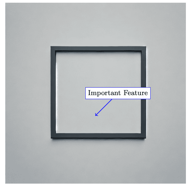
We can move around the node at (5, 4) or label at (4, 3) to match the exact area on the image that we wish to highlight.

8. Scaling and Accuracy Issues

When we place images in LaTeX, scaling can affect the coordinate system TikZ uses.

If we use width=10cm to scale the image, and it collides with its aspect ratio or resolution, we may need to adjust the coordinate alignment manually.

It’s sometimes helpful to measure the final width and height as they appear in the compiled PDF and map the coordinates accordingly.

However, we can also do the following to make it easier for us:

\begin{tikzpicture}[x=1mm,y=1mm]
  \node[anchor=south west, inner sep=0] (img) at (0,0){
    \includegraphics[width=100mm]{example-image.png}
  };
  % Now, each 1 TikZ unit in x or y is 1 mm on paper
  % We can place shapes accordingly
\end{tikzpicture}

By ensuring our tikzpicture has [x=1mm,y=1mm] and the image is width=100mm, we achieve a one-to-one mapping of millimeters from TikZ coordinates to the units on the scaled image. This level of granularity should be sufficient to simplify pinpointing exact locations.

8.1. Temporary Grid

Sometimes, we want a quick way to visualize our coordinate system and decide where to place shapes or labels. Adding a temporary grid can help us see which x and y values might work best.

We can do this by drawing a grid in TikZ and removing it once we’re confident about the positions. For example:

\begin{tikzpicture}[x=1mm,y=1mm]
  % 1) Place the image at (0,0)
  \node[anchor=south west, inner sep=0] (img) at (0,0)
        {\includegraphics[width=100mm]{example-image.png}};

  % 2) Determine the upper-right corner of the image node
  \path (img.north east) coordinate (imgNE);

  % 3) Draw a light grid from (0,0) to (imgNE)
  \draw[step=10,lightgray,very thin] (0,0) grid (imgNE);

  % 4) Example annotation: a red circle at (20,10)
  \draw[red, thick] (20,10) circle (3);

  % 5) A label near the circle
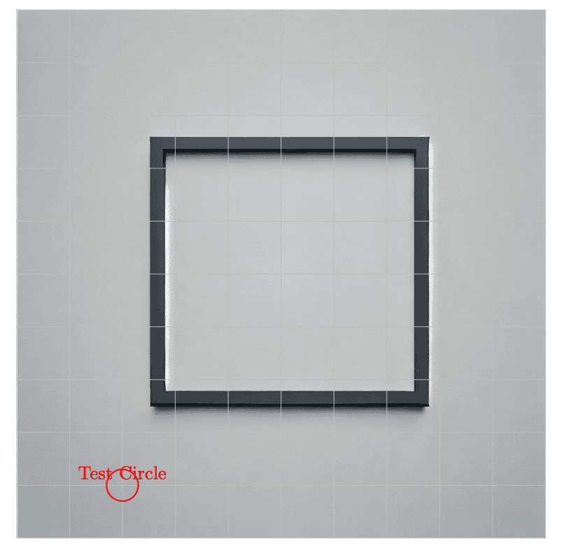
  \node[above, red] at (20,10) {Test Circle};
\end{tikzpicture}

In this snippet:

• We use x=1mm, y=1mm so that each unit in TikZ corresponds to 1 mm in the final document.
• The image is placed in a node called (img) and anchored at (0,0).
• We then use \path (img.north east) coordinate (imgNE); to capture the upper-right corner of the image’s bounding box in the coordinate (imgNE)
• We draw a grid from (0,0) to (imgNE) in steps of 10 mm using lightgray lines. This gives us a quick reference for where our coordinates are.
• Finally, we place a simple annotation (a red circle at (20,10)) and label it.

Here’s the result:

9. Multi-Layered Annotation

As a more advanced example, let’s combine multiple annotations: a rectangle, a circle, an arrow with text, and a highlight.

Here is a code snippet illustrating a multi-layer approach:

\begin{tikzpicture}[x=1mm, y=1mm]
  % Place the image
  \node[anchor=south west, inner sep=0] at (0,0) {
    \includegraphics[width=100mm]{example-image.png}
  };

  % 1) Rectangle highlighting area from (10,10) to (30,25)
  \draw[thick, orange] (10,10) rectangle (30,25);

  % 2) Circle around point (60,40)
  \draw[red, very thick] (60,40) circle (5);

  % 3) Arrow from label node to circle center
  \node[draw=white, fill=white, text=red, font=\bfseries] (circLabel) at (75,40) {Circle Region};
  \draw[->, red, thick] (circLabel) -- (60,40);

  % 4) Another label for the orange rectangle
  \node[draw=white, fill=white, text=orange] at (20,28) {Highlighted Rect};

\end{tikzpicture}

Breaking down the above:

• We set the coordinate system such that each 1 unit in x or y is 1 mm.
• The image is placed at the origin, scaled to be 100 mm wide.
• We draw an orange rectangle in the lower-left region, between (10, 10) and (30, 25).
• We draw a red circle with a radius of 5 mm around the coordinate (60, 40).
• Then, we place a node labeled Circle Region at (75, 40) with a red arrow pointing to the circle center.
• Finally, we add a text label Highlighted Rect above the rectangle in orange.

This produces an image with multiple highlight markers:

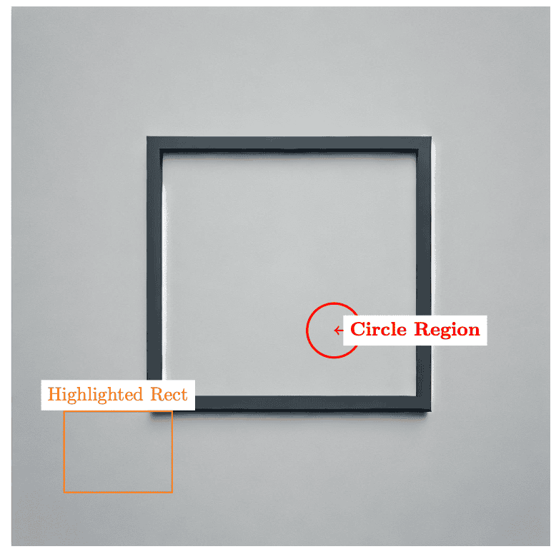
By layering shapes and text, we can convey detailed information directly on the figure.

10. Tips for Accuracy and Maintenance

We can keep our code readable while accurately placing shapes and labels with careful planning:

• Use references or measured distances: if we know the exact size or measure it from a vector file, we can match coordinates precisely.
• Keep code modular: place the image insertion in one piece of code and the annotation in another; this can make adjustments easier.
• Document our coordinates: if the image changes or we swap images, the coordinate system might shift.
• Check the aspect ratio: if we scale images differently in x vs. y directions, we must account for that in our TikZ coordinate system (e.g., using [xscale=2, yscale=1] or similar).
• Use drawing libraries: TikZ is a deep library with many shapes, patterns, arrows, and libraries (like shadows, arrows.meta, calc, and more) that can enhance our annotations.

11. Conclusion

In this article, we discussed how drawing on an image with TikZ gives us a powerful way to create annotated figures and detailed explanations right within LaTeX. By embedding an image in a tikzpicture, we can position circles, rectangles, arrows, and text wherever we need them. Options such as overlay and remember picture offer additional flexibility for combining standard figure environments with TikZ overlays.

Whether highlighting parts of a circuit diagram, pointing to elements in a software interface screenshot, or labeling features in a scientific photograph, TikZ’s coordinate system and styling options allow us to produce professional-looking results. While adjusting coordinates can be a learning curve, we unlock a robust method of visually communicating ideas once we grasp the basics.

With the examples provided, we can confidently start annotating images. We can also explore additional TikZ libraries, such as calc for coordinate arithmetic or arrows.meta for advanced arrow tip, to make our figures even more expressive. Ultimately, the key is experimenting, measuring carefully, and iterating until our images and annotations align perfectly.