

Learn through the super-clean Baeldung Pro experience:
>> Membership and Baeldung Pro.
No ads, dark-mode and 6 months free of IntelliJ Idea Ultimate to start with.
Learn through the super-clean Baeldung Pro experience:
>> Membership and Baeldung Pro.
No ads, dark-mode and 6 months free of IntelliJ Idea Ultimate to start with.
In this tutorial, we’ll cover Splay Tree (ST). It’s a self-adjusting variant of the Binary Search Tree (BST). ST keeps no additional information in nodes needed for the tree balancing.
ST doesn’t put a strong condition on its structure to be always balanced. Instead, it uses heuristics to move the last accessed element to the root of the tree in the hope that it has a higher probability of being accessed later. Thus, the last accessed elements get placed near the root of the tree.
The essential basis of ST is the splaying operation. It’s used to move the last accessed element to the root.
The purpose of splaying is to move the element of interest to the root of the tree. Splaying consists of a series of rotations. Three types of rotations are used in splaying: zig, zig-zig, and zig-zag.
We perform the zig rotation when the splayed element is a direct child of the root. Zig is the terminal step in splaying, as after performing it, the element appears in the root. The example below shows an example of a zig rotation when the splayed element is the left child of the root. This is the right zig rotation. The splayed element is  , and its parent is
  . The nodes are depicted with small circles, while subtrees are depicted with big circles:
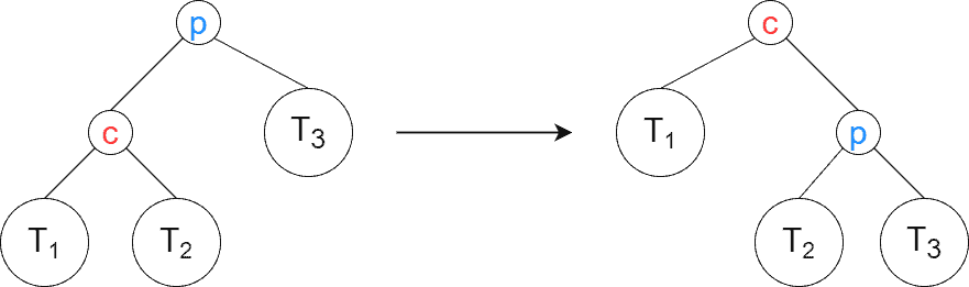
As we see, gets moved to the root, and the previous root becomes its right child. Additionally, the right subtree of becomes the left subtree of .
Below we can see the left zig rotation. Again, the element to be splayed is :
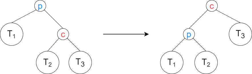
The left and right zig rotations are symmetrically identical.
Let’s write the pseudocode for the zig rotation:
algorithm ZigRotation(p, c):
    // INPUT
    //    p = parent node
    //    c = child node
    // OUTPUT
    //    Zig rotation is performed and c is returned

    if c = p.left:
        p.left <- c.right
        c.right <- p
    else:
        p.right <- c.left
        c.left <- p

return cZig-zig and zig-zag are double rotations. We have the zig-zig case when the splayed element and its parent are both either left or right children. First, we perform the rotation of the parent. Then we rotate the element of interest. The image below shows the zig-zig rotation in action. We’ve depicted the case when the element and its parent are both left children. The splayed element is , its parent is , and its grandparent is  :
:
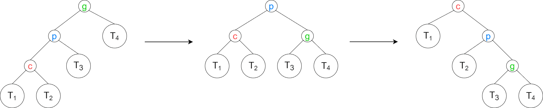
First, the edge connecting with is rotated right. Then, the edge connecting with is rotated right. The case when the splayed element and its parent are both right children is symmetrically identical to the left children case so that we won’t depict it again.
The pseudocode for the zig-zig rotation takes the form:
algorithm ZigZig(g, p, c):
    // INPUT
    //    g = grandparent node
    //    p = parent node
    //    c = child node
    // OUTPUT
    //    Returns the child node c after a zig-zig rotation.

    isLeft <- true
    parentOfG <- g.parent

    if parentOfG != null and g = parentOfG.right:
        isLeft <- false

    p <- Zig(g, p)
    c <- Zig(p, c)

    if parentOfG != null:
        if isLeft = true:
            parentOfG.left <- c
        else:
            parentOfG.right <- c

    return c
Besides the rotations, we also need to take care of assigning to the previous parent of .
The last type of rotation is zig-zag. It’s the case when the element to be splayed is the left child, and its parent is the right child or vice versa. During the zig-zag rotation, the element of interest is rotated twice – first with its parent, then with its new parent. Below, we’ve shown the case when the splayed element is the right child, and its parent is the left child. Again, the splayed element is , its parent is , and its grandparent is :
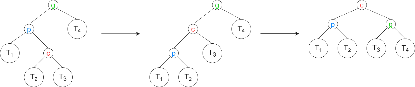
In the first step, the edge connecting with is rotated left. Then, the edge connecting with is rotated right. The symmetric case of being the right child and being the left child is identical to the observed case.
Finally, let’s provide the pseudocode for the zig-zag rotation:
algorithm ZigZagRotation(g, p, c):
    // INPUT
    //    g = grandparent node
    //    p = parent node
    //    c = child node
    // OUTPUT
    //    Zig-zag rotation is performed and c is returned

    isLeft <- true

    if p = g.right:
        isLeft <- false

    c <- Zig(p, c)

    if isLeft = true:
        g.left <- c
    else:
        g.right <- c

    isLeft <- true
    parentOfG <- g.parent

    if parentOfG != NULL and g = parentOfG.right:
        isLeft <- false

    c <- Zig(g, c)

    if parentOfG != NULL:
        if isLeft = true:
            parentOfG.left <- c
        else:
            parentOfG.right <- c

    return c
First, we rotate with , and make a child of . Then, we rotate with , and becomes a child of ‘s previous parent.
Having the pseudocodes for various types of rotations, we can now implement the splaying operation. Splaying accepts a 1-indexed array of nodes representing the path from the root to the element of interest. The first element of the array is the root, and the last element is the splayed element:
algorithm Splay(path):
    // INPUT
    //    path = array of nodes representing the path
    // OUTPUT
    //    The last element of path is splayed along the nodes in path, and the new root is returned

    i <- path.length
    c <- path[i]
    i <- i - 1

    while i > 0:
        p <- path[i]
        i <- i - 1

        if i = 0:
            c <- ZIG(p, c)
            return c
        else:
            g <- path[i]
            i <- i - 1
            leftParent <- true

            if p = g.right:
                leftParent <- false

            leftChild <- true

            if c = p.right:
                leftChild <- false

            if leftParent = leftChild:
                c <- ZigZig(g, p, c)
            else:
                c <- ZigZag(g, p, c)

    return c
At each iteration, the function performs a rotation to move up the tree. If at least two elements remain in the path, then either zig-zig or zig-zag rotation is performed. Otherwise, if a single element is left, then the final zig rotation is performed, and the splayed element is returned. If no elements are left in the path, the function returns the splayed element.
The image below shows the flow of splaying the element with value 12. The splayed element and the rotation edges at each step are colored in red. The current parent is colored in blue, and the current grandparent is colored in green:
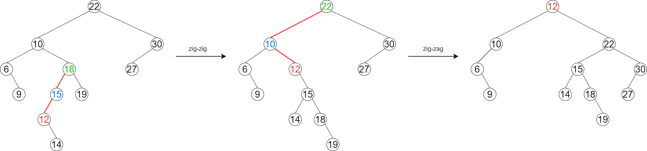
To splay the element of interest in this example, we actually perform one zig-zig, followed by a zig-zag rotation. As we see, the element gets moved to the root at the end of the process. Additionally, the BST invariant is preserved, and the tree has become relatively balanced.
ST supports all the standard operations supported by any BST: insertion, removal, and search. Besides, ST also supports two additional operations: join and split. ST is a very interesting data structure in the sense that all its operations can be implemented using the splaying operation.
The search operation is the same as for any BST. We search for the element down the tree until we find it or until we reach a null node and confirm that the element is absent in the tree. Additionally, we perform splaying on the found element to move it to the root. When the element is absent, we splay the last non-null node in the search path.
Let’s implement a recursive search function that actually performs the lookup. Then, we’ll provide a higher-level search function that wraps the actual search plus splaying:
algorithm RecursiveSearch(r, element, path):
    // INPUT
    //    r = root of ST
    //    element = the element to search for
    //    path = an array of nodes to be populated
    // OUTPUT
    //    The node containing element or the last non-null node
    //    in the search path if element is not in the tree.

    Append r to path

    if r.value = element:
        return r

    if r.value < element:
        if r.right = NULL:
            return r
        else:
            return RecursiveSearch(r.right, element, path)

    if r.left = NULL:
        return r

    return RecursiveSearch(r.left, element, path)
We can now implement the higher-level search:
algorithm Search(r, element):
    // INPUT
    //    r = Root of the Splay Tree (ST)
    //    element = the element to search for
    // OUTPUT
    //    Returns true if element is found and false otherwise.
    //    If element is found, it can be accessed at the root.

    path <- initialize a resizable array
    node <- RecursiveSearch(r, element, path)
    found <- true

    if node.value != element:
        found <- false

    r <- Splay(path)
return foundInsertion can be implemented in two ways. The first version inserts the element into the tree using the ordinary BST insertion. Then it splays the newly inserted element. The second version makes use of the split operation to get two separate trees out of the original tree, with the inserted element acting as the split point. Then, the inserted element becomes the root, and the split trees become its children:
Let’s write the pseudocode of the insertion operation:
algorithm InsertionUsingSplit(r, element):
    // INPUT
    //    r = the root of ST
    //    element = the element to insert
    // OUTPUT
    //    element is inserted into ST, and the new root is returned

    (leftTree, rightTree) <- Split(r, element)
    node <- initialize a new tree node
    node.value <- element
    node.left <- leftTree
    node.right <- rightTree

return nodeWe can use the join operation to implement element removal. First, we perform a search of the element to move it to the root. If the search doesn’t find the element, then there’s no need to remove it. Otherwise, we return a new tree which is the result of joining the left and right subtrees of the original tree:
And the pseudocode is below:
algorithm RemoveUsingJoin(r, element):
    // INPUT
    //    r = the root of the Splay Tree
    //    element = the element to remove
    // OUTPUT
    //    The element is removed from the Splay Tree if it is present, and the new root is returned

    found <- Search(r, element)

    if found = false:
        return

    r <- Join(r.left, r.right)
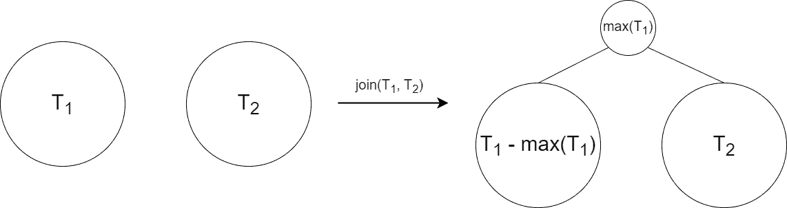
return rThe join operation is defined in the following way. We have two BSTs,  and
and  , where the elements of are less than the elements of . The join operation unites the two trees into a new BST
  , where contains all the elements of and .
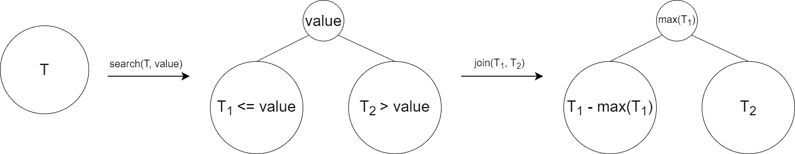
To perform join, we first search for the largest value of . By doing that, we splay it to the root of . As the largest element is now at the root of , the root doesn’t have a right subtree. The join completes by treating as the right child of ‘s root. Let’s write the pseudocode of the join operation:
The join’s pseudocode is written below:
algorithm Join(t1, t2):
// INPUT
// t1 = the root of the first BST
// t2 = the root of the second BST
// OUTPUT
// The new BST is returned, which is the result of joining the input trees.
max <- t1.value
node <- t1.right
while node != NULL:
max <- node.value
node <- node.right
Search(t1, max)
newRoot <- t1
newRoot.right <- t2
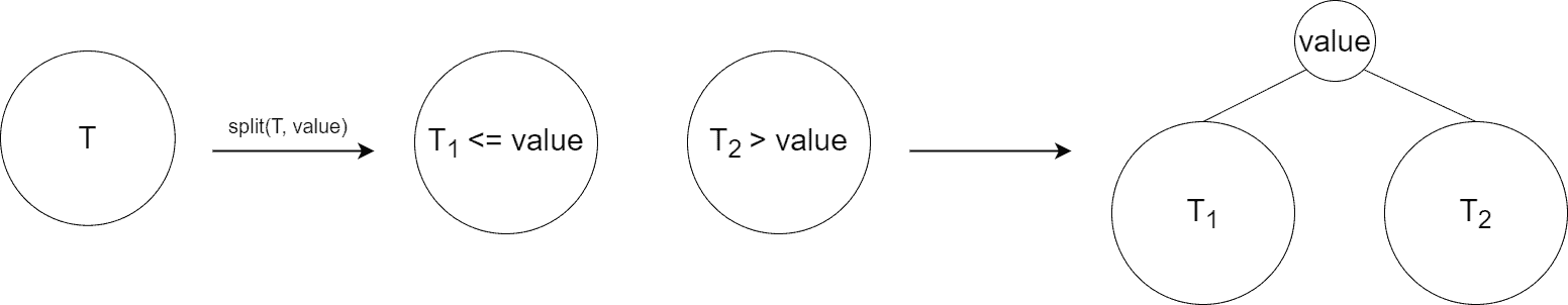
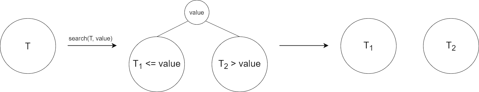
return newRootThe split operation divides a tree into two separate trees and using a split value  . The elements of are less or equal to , and the elements of are greater than :
Finally, let’s provide the split operation’s pseudocode:
algorithm Split(r, split):
    // INPUT
    //    r = the root of the Splay Tree (ST)
    //    split = the element to split the tree
    // OUTPUT
    //    Two BST trees are returned, satisfying the split condition.

    Search(r, split)

    leftTree <- initialize a new tree node
    rightTree <- initialize a new tree node

    if r.value <= split:
        leftTree <- r
        rightTree <- r.right
    else:
        leftTree <- r.left
        rightTree <- r

return (leftTree, rightTree)We’ll just discuss the ready results and won’t dig into the details of the complexity analysis. The interested reader may check out the paper of the data structure inventors for it: Self-Adjusting Binary Search Trees, by R. Tarjan and D. Sleator.
ST doesn’t guarantee worst-case bounds for its operations. The operations are estimated using amortized analysis. Actually, only splaying needs to be estimated, as the rest of the operations are based on it.
It appears that the sequence of  operations on an
  -element ST takes
  time. Thus, the average performance of a single operation is estimated by
  .
.
In this discussion, we’ve covered the Splay Tree data structure. It’s a very practical BST variant and easy to implement. Additionally, it doesn’t consume additional memory needed to store balancing information. Finally, it shows good results in practice when the purpose is to have a good performance in the long run.