External Sorting vs Internal Sorting

1. Introduction

In this tutorial, we’ll discuss the difference between internal and external sort.

2. Difference Between Internal and External Sort

If the data sorting process takes place entirely within the Random-Access Memory (RAM) of a computer, it’s called internal sorting. This is possible whenever the size of the dataset to be sorted is small enough to be held in RAM.

For sorting larger datasets, it may be necessary to hold only a smaller chunk of data in memory at a time, since it won’t all fit in the RAM. The rest of the data is normally held on some larger, but slower medium, like a hard disk. The sorting of these large datasets will require different sets of algorithms which are called external sorting.

3. Algorithms Used for Internal Sort

Following are few algorithms that can be used for internal sort:

3.1. Bubble Sort:

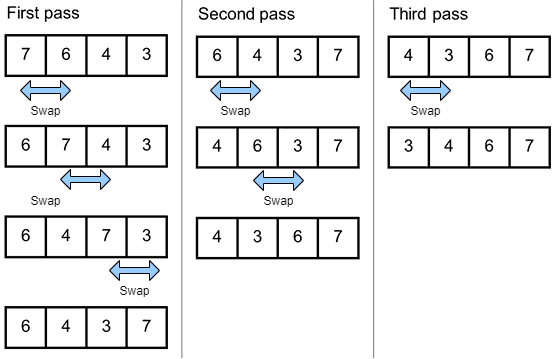
It’s a simple sorting algorithm that repeatedly steps through the list, compares adjacent elements, and swaps them if they’re in the wrong order. More about it can be found in another article:

The algorithm loops through the list until it’s sorted:

3.2. Insertion Sort:

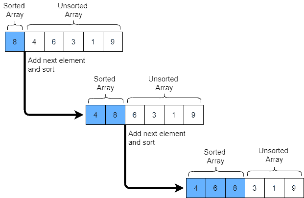
This sorting algorithm works similarly to the way to sort playing cards. The dataset is virtually split into a sorted and an unsorted part, then the algorithm picks up the elements from the unsorted part and places them at the correct position in the sorted part as shown below:

To learn more, please check our article.

3.3. Quick Sort:

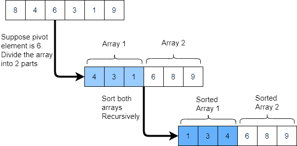
This sorting algorithm picks up a pivot element, then partitions the dataset into two sub-arrays, one sub-array is greater than the element and another sub-array is less than the element. The same process is repeated for sub-arrays till the dataset is sorted as shown below:

Please check our article to learn more. The space complexity of all these algorithms is O() which means that the space requirement goes up with the size of the dataset.

4. Algorithms Used for External Sort

External sort requires algorithms whose space complexity doesn’t increase with the size of the dataset. While the space complexity of Merge Sort is O(), we can optimize it to O()

4.1. Data-flow Diagram

The following diagram has the high-level data flow to sort a large dataset of 50 GB using a computer with RAM of 8GB and Merge Sort Algorithm:

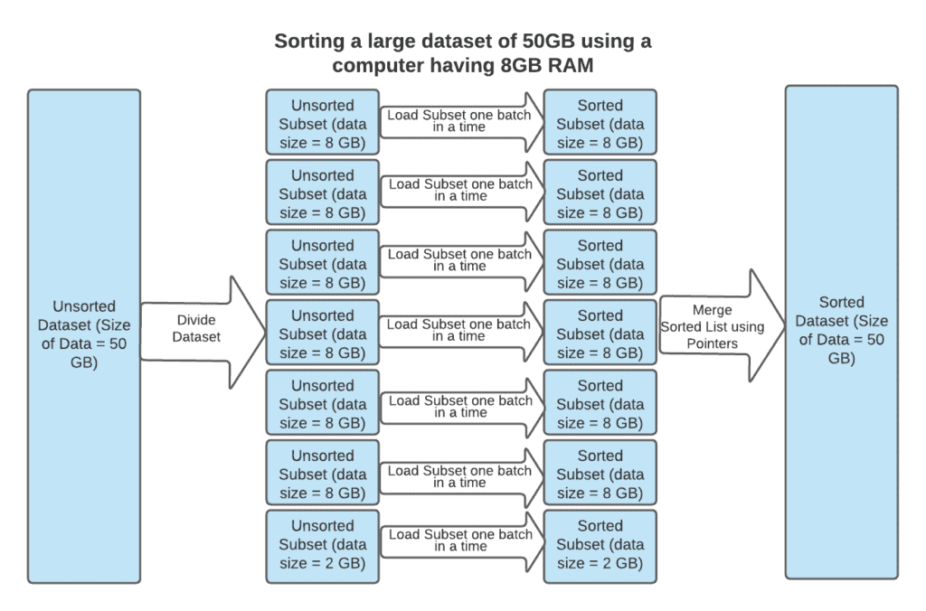
It contains the following steps:

• Divide the large dataset into smaller subsets of size less than 8GB as the RAM of the computer is 8GB. The space complexity of this step is O() as it doesn’t increase with the size of the dataset.
• Use any of the popular internal sorting algorithms to sort the subsets one batch at a time. The space of complexity of these algorithms is O(). The size of these subsets is less than 8GB, it’ll require the same amount of memory to sort them.
• Iterate using pointers to merge sorted subsets. During this, we compare the values of elements of current pointers to subsets and put the smallest value in the output list. Then move the pointer to the next item of the subset which has the smallest value. Since we use pointers, the space complexity of this step is O() and it doesn’t increase with the size of the dataset.

4.2. Step by Step Using an Example

We’ll process the following example using this method:

A S O R T I N G A N D M E R G I N G E X A M P L E

We’re assuming that the computer can store 10 elements.

The first step would be to divide the dataset into 3 subsets and they’re loaded in an external disk.

• A S O R T I N G A N
• D M E R G I N G E X
• A M P L E

Then, as a part of step 2, we’d:

• Load 1^st subset(A S O R T I N G A N) to the computer RAM and sort it to (A A G I N N O R S T). Then store it on an external disk.
• Load 2^nd subset(D M E R G I N G E X) to the computer RAM and sort it to (D E E G G I M N  R  X). Then store it on an external disk.
• Load 3^rd subset(A M P L E) to the computer RAM and sort it to (A E L M P). Then store it on an external disk.

Then, finally:

Initialize the 3 pointers (one each input subsets) and 1 for output. Pointer for 1^st Subset, 2^nd Subset, and 3^rd Subset is 1. Also, the pointer for the output dataset is 1.

• Load the elements as pointed by pointers to three sorted datasets to Computer RAM. It’ll load max 3 elements as there are 3 subsets. It’ll load (A D A) to Computer RAM.
• Find the lowest value from these elements and load it to the output array at the location identified by the output pointer. Since A is lowest in (A D A), load A to output in external disk.
• Increase output pointer by 1 and also increase the pointer of the dataset that has the lowest element by 1. So we’ve to increase the pointer to 1^st subset to 2 and the output dataset to 2. Pointer to 2^nd dataset and 3^rd dataset remains at 1.
• Repeat the steps outlined in b, c, and d. Now since pointers of 1^st subset, 2^nd subset and 3^rd subset is 2,1,1 respectively, it’ll load (A D A) from the external disk to RAM. The lowest value of (A D A) is A which will be stored as 2^nd element of the output dataset. The value of pointers will be increased again, the value of pointers for 3 subsets after the second iteration will be 2,1,2 respectively and pointer for output will be 3.
• These steps will continue till all the elements from the three subsets are processed. The output will be following after all the elements are processed:

A A A D E E E G G G I I L M M N N N O P R R S T X

5. Conclusion

In summary, we use internal sorting when the dataset is relatively small enough to fit within the RAM of the computer and external sorting when the dataset is large and it utilizes algorithms that have minimum space complexity.