How to Calculate the Regularization Parameter in Linear Regression

1. Introduction

In this tutorial, we’ll introduce the classic machine algorithm known as linear regression. First, we’ll discuss the term regression and all the different types of regression. Then we’ll dive into a detailed examination of linear regression, and why we need regularization. Everything will be followed by appropriate mathematical formulas and notations, with a clear explanation of them.

After all, linear regression is one of the most popular and most used statistical and machine learning algorithms, and it’s covered in every related course.

2. Regression

Generally, regression is a family of statistical algorithms that we use to measure relationships between two or more variables. The main logic is that we want to find a connection between input variables (features), which we call independent variables, and outcome or dependent variables. By leveraging this relationship between input and output variables, regression is broadly used as a machine learning model for predicting or forecasting.

For example, we can use R-squared to measure the relationship between two variables, which tells us how close our variables are to the fitted regression line. We can also use polynomial regression to forecast future prices based on historical data, or logistic regression to model the probability for binary classification.

2.1. Types of Regression

There are many types of regression, but here we’ll only mention some of them. Based on the number of input variables, we can classify regression into two groups:

Simple regression – uses only one variable as an input
Multiple regression – uses two or more variables as an input

Similarly, based on the number of dependent or output variables, we can classify regression as:

Univariate regression – there’s only one dependent variable
Multivariate regression – there are two or more dependent variables

The three most commonly used regression models are:

Linear regression – it assumes that we have a linear relationship between input and output variables, and a linear function is used to explain that relationship
Polynomial regression – similar to linear regression, but uses polynomials to approximate the relationship between variables
Logistic regression – uses a logistic function or sigmoid to model a probability for binary classification problems

Finally, it’s worth mentioning that the term regression is also widely used in a different context, as a class of machine learning algorithms. Usually, we can see that most machine learning problems are divided into two classes:

Classification problems – the goal is to predict a predefined label or class. For example, to predict if the sentiment of the particular sentence is positive, or predict the handwritten digit on the image
Regression problems – the goal is to quantify. For example, to predict tomorrow’s price of Tesla stock, or predict the exact temperature using some weather data

3. Linear Regression

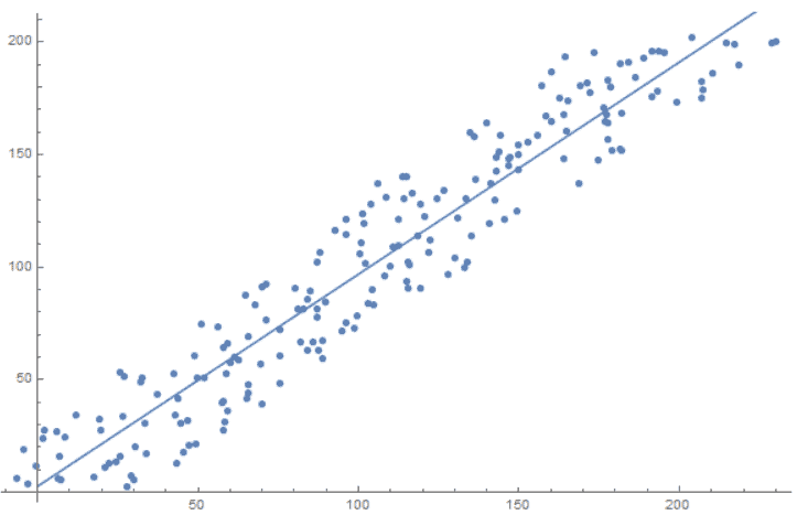
We previously mentioned some of the most used regression techniques, and in this section, we’ll introduce what may be the most popular one. Linear regression is an approach to modelling the relationship between one dependent variable and one or more explanatory variables, either continuous or discrete. This technique helps in predicting the future values of one variable through the use of another variable. It enables us to predict how much weight one variable has on another variable by using the past data of both variables.

The image below shows how linear regression approximates the relationship between features on the $x$ and $y$ axis:

We define linear regression with the formula:

(1) $\begin{equation*} \hat{y} = \theta_{0} + \theta_{1}x_{1} + \theta_{2}x_{2} + ... + \theta_{n}x_{n}, \end{equation*}$

Here, $\hat{y}$ is the predicted value, $n$ is the number of features, $x_{i}$ is the $i$ -th feature value, and $\theta_{j}$ is the $j$ -th model parameter or weight. Also, $\theta_{0}$ is known as a bias term.

Similarly, we can write the equation above using a vectorized form:

(2) $\begin{equation*} \hat{y} = \boldsymbol{\theta}^{T} \cdot \boldsymbol{x}, \end{equation*}$

Here, $\boldsymbol{\theta}^{T}$ is the transpose model’s weight vector, $\boldsymbol{\theta} = (\theta_{0}, \theta_{1}, ..., \theta_{n})$ , and $\boldsymbol{x} = (x_{0}, x_{1}, ..., x_{n})$ is the feature vector, where $x_{0} = 1$ .

Next, to train the model, we first need to measure how well the model fits the training data. For this purpose, we commonly use the mean squared error (MSE) cost function. We define it using the formula:

(3) $\begin{equation*} MSE = \frac{1}{m} \sum_{i=1}^{m} (\boldsymbol{\theta}}^{T} \cdot \boldsymbol{x}^{(i)} - y^{(i)})^{2} \end{equation*}$

Here, $m$ indicates the number of samples, and $y^{(i)}$ is the real value of $i$ -th sample. We use MSE to measure the average squared difference between the estimated values and the real values.

To find the value of $\boldsymbol{\theta}$ that minimizes the cost function, there are three methods:

Closed-form solution
Gradient descent
SVD and Moore-Penrose pseudo inverse

3.1. Closed-Form Solution

By closed-form solution, we mean using a normal equation in order to find the optimal value in only one step. Consequently, we can define the normal equation as:

(4) $\begin{equation*} \hat{\boldsymbol{\theta}} = (\boldsymbol{X}^{T} \cdot \boldsymbol{X})^{-1} \cdot \boldsymbol{X}^{T} \cdot \boldsymbol{y}, \end{equation*}$

Here, $\hat{\boldsymbol{\theta}}$ is an optimal solution of the MSE, $\boldsymbol{X}$ is a matrix that contains all $\boldsymbol{x}^{(i)}$ feature vectors, and $\boldsymbol{y}$ is a vector of target values containing all $y^{(i)}$ .

Since we need to compute the inverse of $(\boldsymbol{X}^{T} \cdot \boldsymbol{X})$ matrix, which is $n \times n$ matrix, where $n$ is number of features, the complexity is around $O(n^{3})$ . As a result, this method can become very slow with the increase in the number of features. In contrast, the complexity is linear regarding the number of samples in the training test.

To conclude, this method isn’t the best approach when we have a lot of features, or too many training samples to fit in memory.

3.2. Gradient Descent

Gradient descent is a technique in machine learning that we usually use in the context of optimization. We use this algorithm to find the minimum of a function by iteratively finding the direction with the steepest slope relative to the current location. In this case, we calculate the steepest slope to the current location using gradient descent.

Specifically, if our MSE cost function $J(\boldsymbol{\theta})$ has a form:

(5) $\begin{equation*} J(\theta) = \frac{1}{m} \sum_{i=1}^{m} (\theta}^{T} \cdot x^{(i)} - y^{(i)})^{2}, \end{equation*}$

Then the gradient is:

(6) $\begin{equation*} \frac{\partial J(\theta)}{\partial \theta} = \frac{2}{m} \sum_{i=1}^{m}[ (\theta}^{T} \cdot x^{(i)} - y^{(i)})x^{(i)}]. \end{equation*}$

After that, we update weights with gradient multiplied by learning rate $\alpha$ :

(7) $\begin{equation*} \theta := \theta - \alpha \cdot \frac{\partial J(\theta)}{\partial \theta}. \end{equation*}$

In our case, this approach leads to a global minimum because our cost function is a convex function, and therefore it has only one local minimum that’s also a global minimum. Gradient descent is prevalent because it’s widely applicable in many machine learning techniques, including neural networks. Despite that, it has some drawbacks.

Because gradient descent is an iterative approach, it can take time to reach the optimum solution. Also, the convergence depends on the learning rate $\alpha$ .

To conclude, gradient descent or modifications of this method are widely used in machine learning, but in our case, there’s an even faster method that we’ll describe below.

3.3. SVD and Moore-Penrose Pseudo Inverse

One step before the normal equation:

(8) $\begin{equation*} \boldsymbol{\theta} = (\boldsymbol{X}^{T} \cdot \boldsymbol{X})^{-1} \cdot \boldsymbol{X}^{T} \cdot \boldsymbol{y}, \end{equation*}$

We have this equation:

(9) $\begin{equation*} \boldsymbol{X}^{T} \cdot \boldsymbol{X}\boldsymbol{\theta} = \boldsymbol{X}^{T} \cdot \boldsymbol{y}. \end{equation*}$

Since this equation almost never has an exact solution, because there are more samples than features, we approximate the $\boldsymbol{\theta}$ vector as close as possible using Euclidean distance:

(10) $\begin{equation*} \min_{\theta} = ||\boldsymbol{X}\hat{\boldsymbol{\theta}} - \boldsymbol{y}||^{2}_{2}. \end{equation*}$

We call this problem Ordinary Least Square (OLS). There are many ways of solving it, and one of them is using the Moore-Penrose pseudo inverse theorem. In particular, it says that for a system of linear equations, $Ax = b$ , the solution with minimal $L2$ norm $||Ax - b||^{2}_{2}$ is $A^{\dagger}b$ , where $A^{\dagger}$ is a Moore-Penrose pseudoinverse.

Following that, we calculate the value $A^{\dagger}$ , or in our example $X^{\dagger}$ , through singular value decomposition (SVD):

(11) $\begin{equation*} X = V\Sigma U^{T} \end{equation*}$

Here, $X$ has the format $n \times m$ , where $n$ is the number of features and $m$ is the number of samples, $V_{n \times n}$ is an orthogonal matrix, $\Sigma_{n \times m}$ is a diagonal matrix and $U_{m \times m}$ orthogonal matrix. Therefore, we calculate the Moore-Penrose pseudoinverse as:

(12) $\begin{equation*} X^{\dagger} = V\Sigma^{\dagger} U^{T} \end{equation*}$

Here, $\Sigma^{\dagger}$ is constructed from $\Sigma$ by taking the reciprocal values of nonzero elements, and transposing the resulting matrix. Finally, to calculate linear regression weights, we use the formula:

(13) $\begin{equation*} \theta = V\Sigma^{\dagger} U^{T}y. \end{equation*}$

This method is used in the Scikit-learn package as a default for linear regression optimization because it’s speedy and numerically stable.

4. Regularization in Linear Regression

Regularization is a technique in machine learning that tries to achieve the generalization of the model. It means that our model works well not only with training or test data, but also with the data it’ll receive in the future. In summary, to achieve this, regularization shrinks the weights toward zero to discourage complex models. Accordingly, this avoids overfitting and reduces the variance of the model.

There are three main techniques for regularization in linear regression:

Lasso Regression
Ridge Regression
Elastic Net

4.1. Lasso Regression

Lasso regression, or L1 regularization, is a technique that increases the cost function by a penalty equal to the sum of the absolute values of the non-intercept weights from linear regression. Formally, we define L1 regularization as:

(14) $\begin{equation*} J(\theta) = \frac{1}{m} \sum_{i=1}^{m} (\theta}^{T} \cdot x^{(i)} - y^{(i)})^{2} + \lambda\sum_{j=1}^{n}|\theta_{j}|, \end{equation*}$

Here, $\lambda$ is a regularization parameter. Basically, $\lambda$ controls the degree of regularization. In particular, the higher the $\lambda$ is, the smaller the weights become. In order to find the best $\lambda$ , we can start with $\lambda = 0$ and measure the cross-validation error at each iteration, increasing the $\lambda$ with a fixed value.

4.2. Ridge Regression

Similar to Lasso Regression, Ridge Regression, or L2 regularization, adds a penalty to the cost function. The only difference is that the penalty is calculated using the squared values of non-intercept weights from linear regression. Thus, we define L2 regularization as:

(15) $\begin{equation*} J(\theta) = \frac{1}{m} \sum_{i=1}^{m} (\theta}^{T} \cdot x^{(i)} - y^{(i)})^{2} + \lambda\sum_{j=1}^{n}\theta_{j}^{2}. \end{equation*}$

Like with L1 regularization, we can estimate the $\lambda$ parameter in the same way. The only difference between Lasso and Ridge is that Ridge converges faster, while Lasso is more commonly used for feature selection.

4.3. Elastic Net Regression

In summary, this method is a combination of the previous two approaches; it combines penalties from both Ridge and Lasso Regression. Therefore, we define Elastic Net regularization with the formula:

(16) $\begin{equation*} J(\theta) = \frac{1}{m} \sum_{i=1}^{m} (\theta}^{T} \cdot x^{(i)} - y^{(i)})^{2} + \lambda_{1}\sum_{j=1}^{n}|\theta_{j}| + \lambda_{2}\sum_{j=1}^{n}\theta_{j}^{2}. \end{equation*}$

In contrast to the previous two methods, here we have two regularization parameters, $\lambda_{1}$ and $\lambda_{2}$ . As such, we’ll have to find both of them.

5. Conclusion

In this article, we explored the term regression, its types, and linear regression in detail. Then we explained the three most commonly used regularization techniques, and the way of finding the regularization parameter. In conclusion, we learned the mathematics behind linear regression and regularization methods.

Full Archive

About Baeldung

Core Concepts

Operating Systems

Artificial Intelligence

Graph Theory

Latex