

Learn through the super-clean Baeldung Pro experience:
>> Membership and Baeldung Pro.
No ads, dark-mode and 6 months free of IntelliJ Idea Ultimate to start with.
Learn through the super-clean Baeldung Pro experience:
>> Membership and Baeldung Pro.
No ads, dark-mode and 6 months free of IntelliJ Idea Ultimate to start with.
In this tutorial, we analyze the worst-case, the best-case, and the average-case time complexity of QuickSelect. It’s an algorithm for finding the  -th largest element in an
  -element array (
 ). In honor of its inventor, we also call it Hoare’s Selection Algorithm.
QuickSelect is similar to QuickSort. The main difference is that the sorting algorithm recurses on both subarrays after partitioning, whereas the selection algorithm recurses only on the subarray that provably contains the -th largest element:
algorithm QuickSelect(a, ℓ, h, k):
// INPUT
// a = an n-element array
// ℓ = the start index of the subarray (initially, ℓ = 1)
// h = the end index of the subarray (initially, h = n)
// OUTPUT
// The k-th largest element in a
if ℓ = h:
return a[ℓ]
else if ℓ < h:
p <- choose the pivot, partition a[ℓ:h], and return the new index of the pivot
if k = p:
return a[p]
else if k < p:
return QuickSelect(a, ℓ, p-1, k) // Apply QuickSelect to the left subarray
else:
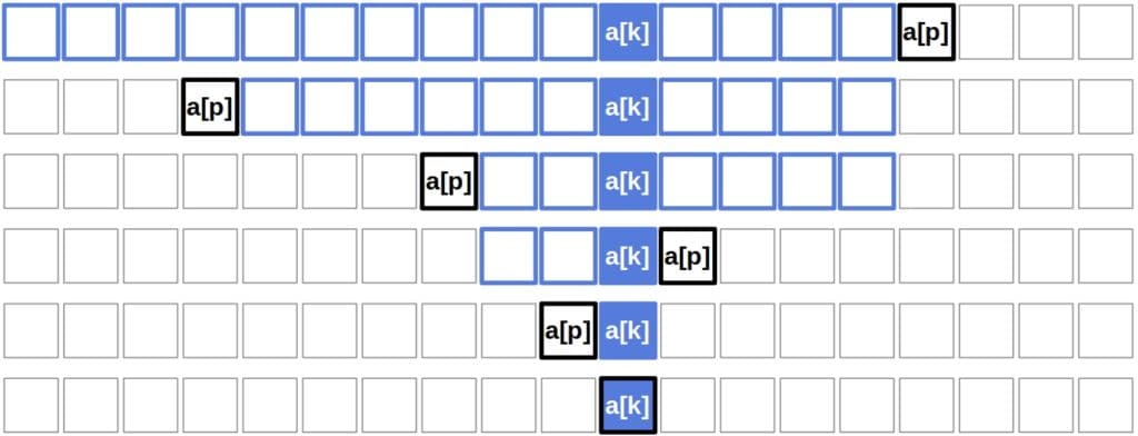
return QuickSelect(a, p+1, h, k) // Apply QuickSelect to the right subarrayWe can nicely visualize the steps QuickSelect makes while searching:
Algorithm 1 is a generic form of QuickSelect since it doesn’t specify how to partition the input array and select pivot elements. Several methods have appeared over the years. Since it’s the easiest to analyze, we’ll use Lomuto partitioning with random pivot selection in this tutorial. Other approaches have the same or a similar complexity or can be analyzed similarly.
In brief, Lomuto selects a random element in the input array ![a[\ell:h]](/wp-content/ql-cache/quicklatex.com-7c8e12cf14287a77ef263c8a017087c9_l3.svg "Rendered by QuickLaTeX.com") as the pivot, swaps it with the last element
as the pivot, swaps it with the last element ![a[h]](/wp-content/ql-cache/quicklatex.com-0f2d67fab1b7161243fb1dd2893882f5_l3.svg "Rendered by QuickLaTeX.com") , and splits the array in a single loop iterating from
, and splits the array in a single loop iterating from ![a[\ell]](/wp-content/ql-cache/quicklatex.com-2bdeddf6455885cc502d3b65a0d1f831_l3.svg "Rendered by QuickLaTeX.com") to
to ![a[h-1]](/wp-content/ql-cache/quicklatex.com-fb20d465735626cb7d8a04e266f76bbf_l3.svg "Rendered by QuickLaTeX.com") :
:
algorithm LomutoPartitioning(a, ℓ, h):
    // INPUT
    //    a = an n-element array
    //    a[ℓ:h] = the subarray a[ℓ], a[ℓ+1], ..., a[h] (ℓ < h)
    // OUTPUT
    //    k = the pivot's index that splits a[ℓ:h] into left and right subarrays

    Randomly select r from {1, 2, ..., n}
    Swap a[h] with a[r]

    x <- a[h]
    k <- ℓ - 1

    for j <- ℓ to h - 1:
        if a[j] <= x:
            k <- k + 1
            Swap a[j] with a[k]

    Swap a[k + 1] with a[h]

return k + 1Before deriving the complexity bounds of the worst-case scenario, let’s first determine its structure.
We see that QuickSelect discards a portion of the original array in each recursive call. The worst-case corresponds to the longest possible execution of the algorithm. It’s the one in which the -th largest element is the last one standing, and there are recursive calls. A necessary condition for that is that QuickSelect discards the smallest possible portion in each call. In other words, the subarray it ignores should be empty so that it discards only the current pivot. Additionally, the pivot shouldn’t be the -th largest element. Mathematically, each recursive call should fulfill either of the two conditions:
 and
and 
 and
and 
However, they aren’t sufficient for the worst case to occur. Let’s say that we approach the sought element always from the right. As a result, we make  recursive calls before we find it. On the other hand, we make calls if we approach it only from the left. This is the worst-case scenario only if
  or
or  , respectively. If
  , then to find the -th largest element in the -th call, the algorithm should select all the other elements as pivots before reaching it. So, QuickSelect approaches the element from both sides in the worst case if .
Lomuto partitioning of an -element array performs  comparisons and at most swaps. So, its complexity is
  . Let’s denote as
  the number of steps (comparisons and swaps) QuickSelect performs when searching an -element array. Since QuickSelect always reduces the size of the subarray to recurse on by
  (because the ignored subarray is empty and the pivot isn’t included in the other subarray), the following recurrence holds:
(1) 
Unfolding it, we get:
![\[\begin{aligned} T_n &= \Theta(n) + Theta(n-1) + \ldots + \Theta(1) \\ &= \Theta\left(n+(n-1)+\ldots+1\right) \\ &=\Theta\left(\frac{n(n+1)}{2}\right) \\ &=\Theta(n^2) \end{aligned}\]](/wp-content/ql-cache/quicklatex.com-5ab7c7b3535e376a2f6ed2a0509968e7_l3.svg "Rendered by QuickLaTeX.com")
So, QuickSelect is of quadratic complexity in the worst case.
The best-case occurs when QuickSelect chooses the -th largest element as the pivot in the very first call. Then, the algorithm performs steps during the first (and only) partitioning, after which it terminates. Therefore, QuickSelect is in the best case.
Before determining the algorithm’s average-case complexity, let’s consider what it means to analyze the average case. To be more precise, by average, we mean expected, which is a term from probability theory.
The expected complexity of an algorithm is the expectation of its complexity over the space of all possible inputs. That is, we regard the input as random and following probability distribution. Then, we find the expectation under that distribution. Usually, we assume the distribution is uniform. That means that we consider all the inputs equally likely.
Even though we don’t know the actual distribution of the inputs the algorithm encounters in the real world, the uniform model is a pretty good choice: the analyses based on it have proved accurate and robust in many cases so far. Moreover, we can introduce randomness through the algorithm to ensure the uniform model holds no matter the input’s underlying distribution. For example, we can randomly shuffle the input array before we call QuickSelect. Or, we can choose the pivots at random. However, if we introduce randomness through the algorithm, then the interpretation of the average case changes.
Under the assumption that the input arrays follow a uniform distribution, the average case describes the complexity averaged over all possible inputs. But, if we randomly shuffle the input array or randomly choose the pivot element, then the average case we analyze describes the complexity averaged over all possible executions of QuickSelect on an input array.
In the case of QuickSelect, we’ll consider only the case with all elements distinct from one another. As we assume that  contains no duplicates, it can be thought of as a permutation of
  , which means that we can work with the numbers from
  instead of abstract elements
 ![a[1], a[2], \ldots, a[n]](/wp-content/ql-cache/quicklatex.com-fbfa2204e227fb4fe1a9d7c063129ad4_l3.svg "Rendered by QuickLaTeX.com") . Switching to is justified because each element
. Switching to is justified because each element ![a[i]](/wp-content/ql-cache/quicklatex.com-42e34b2b8788502423ed7c709a1494a6_l3.svg "Rendered by QuickLaTeX.com") has its unique rank in the range
has its unique rank in the range  and we can disregard the case with the duplicates since it has the same complexity.
Since in each call we choose the pivot randomly, it follows that the pivot’s rank ( ) follows the uniform distribution over
  .
.
We’ll express the expected complexity of QuickSelect in terms of the input size, . We’ll track only the number of comparisons it makes because the number of swaps in each partitioning is bounded from above by the number of comparisons.
Let’s define random variables  :
:
(2) 
The total number of comparisons QuickSelect makes when searching through an array of numbers is then:
(3) 
and the expected, that is, the average number of comparisons for an input of size is:
(4) ![\begin{equation*} \begin{aligned} C_n&=&E\left[\sum_{i=1}^{n-1}\sum_{j=i+1}^{n}X_{i,j}\right] \\ &=& \sum_{i=1}^{n-1}\sum_{j=i+1}^{n}E[X_{i,j}] \\ &=& \sum_{i=1}^{n-1}\sum_{j=i+1}^{n}q_{i,j} \end{aligned} \end{equation*}](/wp-content/ql-cache/quicklatex.com-848cd11feff0e010053b8382a2b99e73_l3.svg "Rendered by QuickLaTeX.com")
where  is the probability that
  . How can we compute ?
There are three cases to consider:


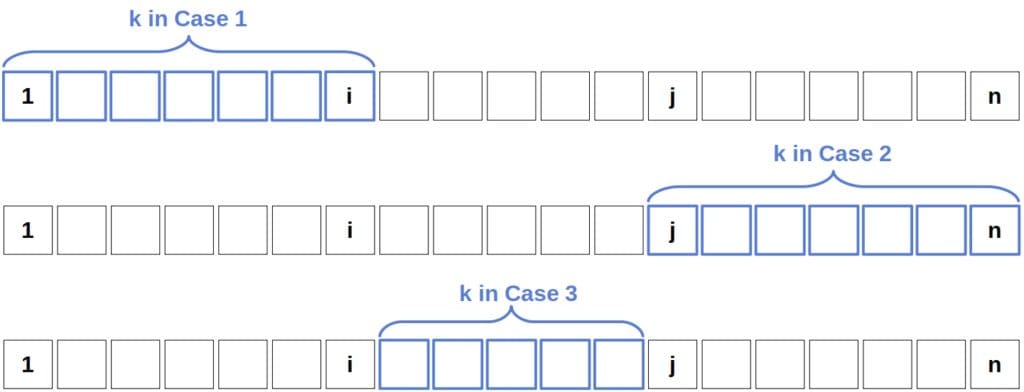
QuickSelect doesn’t compare  and
and  if it selects as a pivot or a number that’s between them. It holds for each of the above three cases. If gets to be the pivot, then the algorithm’s found the number it’s been looking for, so the search stops. If the pivot is between and , then ends up in the left and in the right subarrays during partitioning. Thus, the algorithm can compare only the elements which end up in the same subarray in a call.
But, QuickSelect does compare the pivot element to all the other numbers in a recursive call! So, for  and
and  to get compared, Quickselect should choose or as the pivot before any other number from a range of the corresponding case.
Since the pivots are randomly distributed, the selection probability of any integer from the range ![[\ell, h]](/wp-content/ql-cache/quicklatex.com-9d4388d3aec35261b40d3257160aad0f_l3.svg "Rendered by QuickLaTeX.com") is
is  . Since the selections of and as the first pivot from are mutually exclusive events, we can sum their probabilities to get in each case:
(5) 
We can split  into summations by each case and then add together the obtained sums. In Case 1, we have:
(6) 
We get a similar result for Case 2:
(7) 
Case 3 will also be  :
:
(8) 
We used the definition  . Since
  for all
  , we have:
(9) 
Therefore, QuickSelect is in the average case.
We analyzed QuickSelect that uses Lomuto partitioning, but there are other alternatives such as Hoare partitioning. It scans the input array from both ends. Although it performs slightly more comparisons than Lomuto partitioning, it makes fewer swaps on average. Nevertheless, QuickSelect has the same complexity no matter if we use Hoare or Lomuto partitioning.
We may choose the pivot deterministically in both partitioning schemes, always selecting the first, the last, or whatever element. But, we may also pick it randomly as we did here. Both strategies have the same asymptotic complexity, but random selection may result in faster runtime in practice.
However, there’s a way to reduce the worst-case complexity to , which is to select pivots with a Median of Medians. It’s an algorithm that returns an element that is guaranteed to be smaller than the top 30% and larger than the bottom 30% elements of the input array. That means that we reduce the size of the input array by a factor of 0.7 in the worst case, which gives the following recurrence:
(10) 
and results in the linear worst-case complexity:
(11) 
In this article, we analyzed the worst, best, and average-case time complexity of QuickSelect. The usual implementations of the algorithm, which use Hoare or Lomuto partitioning, is of quadratic complexity in the worst case but is linear in the average and best cases irrespective of the pivot selection strategy. However, using the Median of Medians to select pivots results in the linear runtime even in the worst case.