Learn through the super-clean Baeldung Pro experience:
>> Membership and Baeldung Pro.
No ads, dark-mode and 6 months free of IntelliJ Idea Ultimate to start with.
Last updated: May 5, 2023

Learn through the super-clean Baeldung Pro experience:
>> Membership and Baeldung Pro.
No ads, dark-mode and 6 months free of IntelliJ Idea Ultimate to start with.
One of the common challenges in signal processing is to detect important points in time or in space like peaks. These points represent local maxima (or minima) which usually have proper meaning in a given example.
For instance, let’s imagine a controllable infrared camera where the goal is to automatically move it in a way so that it includes the biggest number of hotspots. In this example, the “hotspot” is a local maxima peak on a 2D image. Therefore, the same problem can be written like “move the camera so that the number of detected peaks is the maximum“.
In this tutorial, we’re going to explore the possible technical solutions for peak detection also mentioning the complexity cost.
The signal can have 1, 2, or more dimensions. In the 1D case, the detection is already not trivial but it becomes more complex if we’d like to do in 2D space. Higher dimensions fall apart from the common applications, even the terminology changes: we cannot speak about peak anymore but hyperdensity.
In addition, the signal can be continuous or quantized. We know continuous signals usually in closed formulas and we have the possibility to evaluate it at any point in the parameter space. Quantized signals – like images – are limited in resolution and parameter range.
In this article, we’re focusing on 2D quantized signals only. That is to say, we’ll talk about images and pixels as data points.
A peak is a position on the image where all the surrounding pixels have a smaller value:
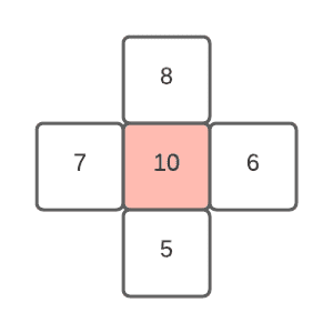
The range of values of a pixel depends on the application and it’s the sensitivity property of the image. For instance, a simple grayscale image uses 8 bit of memory (values between 0 and 255), while scientific applications tend to use 64 bit with the range of 0 to 1.
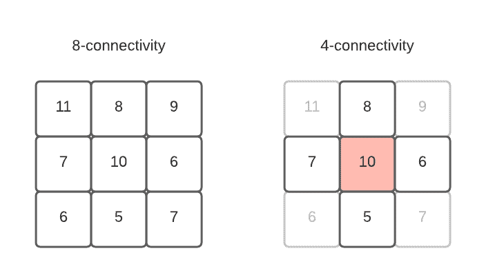
Interestingly, the definition of the “surrounding pixels” is not trivial. We can say there are 4 connected pixels (top, bottom, left, right) or 8 connected pixels (all surrounding ones). To demonstrate the importance of this definition let’s create an example that would be a peak in the case of 4-connectivity but not in 8-connectivity:
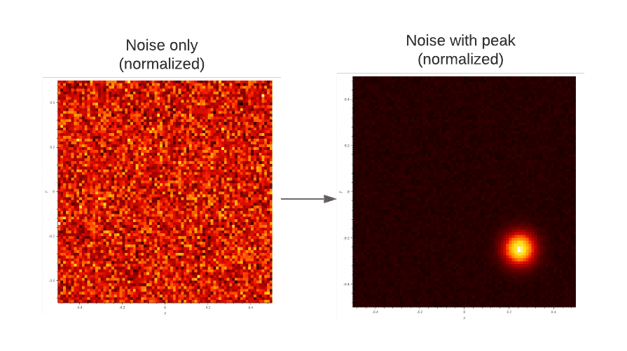
The noise is a general term of unwanted modifications of the signal. Let’s consider the example of our infrared camera. If we happen to point it to a white wall, our image would be homogeneous but due to the noise, there could be many pixel positions labeled as a peak if we take only the definition above. In practice, the peak-to-be-detected spreads on a much bigger area (even if the real peak is only one pixel), which helps to distinguish it from the noise:
In our previous example, we stated “the number of detected peaks” which indicates that we don’t have priory information about how many peaks we expect. Consequently, we can have multiple scenarios that demand different solutions:
 and only number of peaks number of peaks number of peaks
where is a positive natural number.
Apart from the information on how many peaks we expect to have on the image, we might consider the number of peaks we look for.
Let’s consider an image consisting of the pressure value of a pet’s pawn on a surface. The goal is to detect the five toes of the animal. In this example, we look for exactly 5 peaks for further analysis.
There are several approaches to find the desired number of peaks. Each has its own advantage and disadvantage. In the following, we explore some of the most common solutions with their complexities.
If we happen to know that there is one and only one peak, we can simply search for the biggest value on the image, it must be the peak we look for.
This idea requires a simple unsorted search. Hence the complexity is linear  , where
  is the number of columns and
  is the number of rows on the image.
W can use the same idea to detect all the peaks on the image, not just the global one. This requires a bit more work because we have to analyze each position against the definition of the peak. This means we check the values of the surrounding 4 or 8 pixels at each position of the image and label the one which satisfies the definition.
In terms of complexity, we’re still linear () as before but technically it is a little more work to spend at each iteration.
The benefit from the previous method is that we can have all the peak positions on the image, even if some of them come from noise and not a real, desired peak. If we assume that a normal distribution represents well the peak, we can fit a Gaussian curve on it. This has two benefits: we can filter out peaks that don’t resemble the desired distribution (filtering out the  values) and we can refine the position of the peak by resampling with the – already know – distribution.
If we’re ready to sacrifice finding all the peaks and are satisfied only with a peak of the many, we can boost the searching algorithm:
algorithm FindPeak(image):
    // INPUT
    //    image = a 2D matrix representing the image
    // OUTPUT
    //    (i, j) = coordinates of a 2D peak

    m <- image.cols
    j <- m / 2
    (i, j) <- globalMax(j)
    if image[i, j-1] < image[i, j] and image[i, j+1] < image[i, j]:
        return (i, j) // as a 2D-peak
    if image[i, j-1] > image[i, j]:
        return FindPeak(image left to column j)
    if image[i, j+1] > image[i, j]:
        return FindPeak(image right to column j)
Where  is an image with width and height . The
  is the pixel value in row
  and column
  .
.
We start off with the column in the middle and search for the maximum value. At that position, we check if we’re on a peak or not. If not, we check in which direction the value increases and set the new column at the center of the remaining half in that direction and solve the exact same problem on a smaller image. We continue up until we reach one of the peaks. This algorithm ensures that we end up on a peak, but it’s not necessarily the biggest peak.
We can realize that the algorithm doesn’t visit all the columns, so it seems that we do better than the previous algorithm.
Let’s say the complexity needed for this algorithm is  for an image with rows and columns. We can state that:

The  is the cost of searching the global maximum in the column. As the values are not ordered we have to scan the whole column to find the biggest value.
We can also say that if there is only one column left we just need to scan it for the maximum value. This is the worst-case scenario:

Cutting the value by half at each step we maximum have  steps. In conclusion, it means the overall cost of this approach is
  .
.
Depending on the situation we might be able to tell the size of the peak with respect to the resolution of the image. In that case, we can convert the task into a simple pattern matching problem. The cross-correlation is a method to measure the similarities between two signals in different positions relative to each other.
In 2D space it means we define a kernel (the peak) and scan the whole image and calculate the “similarity” for each pixel. This operation is known as convolution. We place the kernel onto all pixels and compute the center value as the “sum-product” of the pixels:
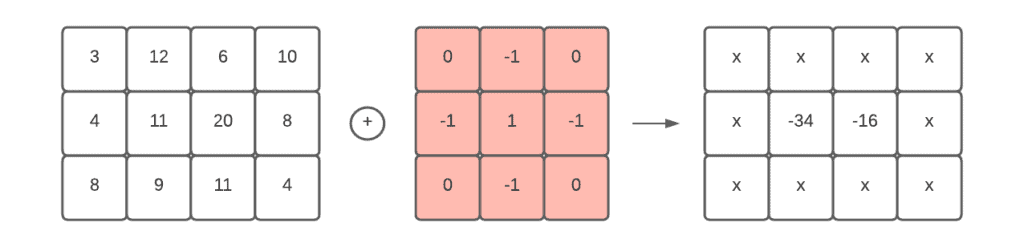
We can see that the “sum-product” gives higher values for those positions that resemble more to the kernel than those that don’t. The final step of this algorithm is to filter out the pixel values that are higher than a given threshold. They potentially represent peaks on the image.
As mentioned above, this algorithm requires parameters (kernel size, threshold) to be tuned for correct detection. This constraint makes this method too rigid and it’s usually avoided.
The simplest implementation of the convolution is scanning the image with the kernel and calculate the new image after the operation. Therefore, it’s easy to realize that the complexity is linear, similarly to the previous ones:
Detecting peaks in an image is a common problem in image processing. In this article, we learned about the characteristic of it and possible solutions. In special cases, more sophisticated algorithms are known and used like the Genetic algorithm or the famous optimization method Gradient Descent. They are appreciated mainly in scientific applications for instance.