

Learn through the super-clean Baeldung Pro experience:
>> Membership and Baeldung Pro.
No ads, dark-mode and 6 months free of IntelliJ Idea Ultimate to start with.
Last updated: February 13, 2025
Learn through the super-clean Baeldung Pro experience:
>> Membership and Baeldung Pro.
No ads, dark-mode and 6 months free of IntelliJ Idea Ultimate to start with.
In this tutorial, we’ll talk about the weight decay loss. First, we’ll introduce the problem of overfitting and how we deal with it using regularization. Then, we’ll define the weight decay loss as a special case of regularization along with an illustrative example.
A very important issue when training machine learning models is how to avoid overfitting. First, we’ll introduce the basic concepts regarding overfitting, which are bias and variance.
We define bias as the difference between the ground truth values and the average predictions of the model during training. As the bias of a model increases, the underlying function it learns becomes simpler since the model pays less attention to the training data. As a result, the model performs poorly on the training set.
On the other hand, variance is defined as the variability of a prediction of the model for a given sample. This means that a model with a high variance has learned a very complex underlying function minimizing the prediction error on the given training set. However, high variance results in low generalization capability to new given data since the model has paid a lot of attention to the training data.
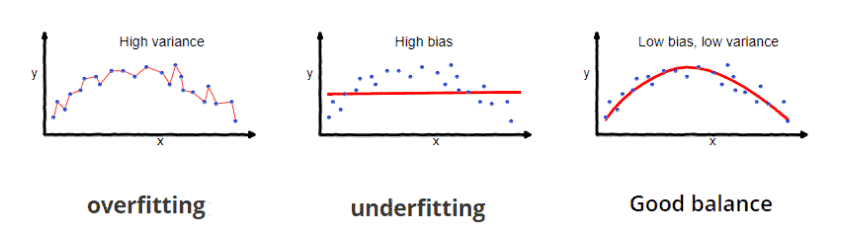
The above definition leads to the well-known bias-variance trade-off in machine learning. On the one hand, you can train a deep learning model with a lot of parameters that can learn a very complex function and achieve high prediction accuracy on the training set. This model will have high variance and low bias and will not be able to generalize to new unseen data. This concept is defined as overfitting.
On the other hand, you can train a model with much fewer parameters in order to learn a simpler function and be able to generalize to new data. This model will have low variance and high bias leading to underfitting.
The ideal scenario is to find a balance between the variance and the bias so as to learn a function as complex as it needs to learn the given task. In the image below, we can see diagrammatically the problem of overfitting:
The most well-known technique to avoid overfitting is regularization. The main idea behind regularization is to force the machine learning model to learn a simpler function in order to reduce the variance and increase the bias.
But, how can we control the complexity of a function? The answer lies in the magnitude of its learnable parameters. When a model learns a very complex function, the magnitude of its learnable parameters is high.
Based on this observation, regularization adds an extra term to the loss function during training that aims to keep the magnitude of the learnable parameters low. As a result, the underlying function that the model learns is simpler, and the variance decreases, preventing overfitting.
There are different types of regularization based on the formula of the regularization term in the loss function. The weight decay loss usually achieves the best performance by performing L2 regularization.
This means that the extra regularization term corresponds to the L2 norm of the network’s weights. More formally if we define  as the loss function of the model, the new loss is defined as:

where  corresponds to the network parameters,
  to the number of samples, and
  is a coefficient that balances the two terms of the loss function. When we increase the value of , we decrease the magnitude of the weights resulting in a simpler underlying function and a lower variance.
Now, let’s see a simple example that illustrates how we train a model with a weight decay loss. We’ll use the task of logistic regression as an example.
The loss function in logistic regression is defined as:

where  and
and  denote the ground truth label and the prediction respectively. So, if we replace
  to the previous equation, we get:

where  corresponds to the input of the model,
  to the learnable weights of the model, and
  to a bias term. To avoid overfitting, we’ll add the weight decay loss and the new loss function will look like this:

In this tutorial, we presented the weight decay loss. First, we described the bias-variance trade-off and how to deal with overfitting using regularization. Then, we defined the weight decay loss along with a simple example.