Merge Two Sorted Arrays Into a Sorted Array | Baeldung on Computer Science

1. Overview

In this tutorial, we’ll discuss how to merge two sorted arrays into a single sorted array and focus on the theoretical idea and provide the solutions in pseudocode form, rather than focusing on a specific programming language.

First, we’ll define the problem and provide an example that explains the meaning of merging two sorted arrays.

Second, we’ll discuss two approaches to solving the problem.

Finally, we’ll compare the provided approaches and discuss the case in which both of them have the same complexity.

2. Defining the Problem

The problem gives us two arrays, $A$ of size $n$ , and $B$ of size $m$ . Both arrays are sorted in the increasing order of their values.

In other words:

$\boldsymbol{A[i] \leq A[i + 1] ; i \in [0, n - 2]}$

$\boldsymbol{B[j] \leq B[j + 1] ; j \in [0, m - 2]}$

After that, the problem asks us to calculate the resulting array $\boldsymbol{R}$ of size $\boldsymbol{n+m}$ that contains all the elements from $\boldsymbol{A}$ and $\boldsymbol{B}$ . Note that, the resulting array $R$ must be sorted as well. In other words:

$\boldsymbol{R[id] \leq R[id + 1] ; id \in [0, n + m - 2]}$

To understand the idea in a better way, let’s take the following example:

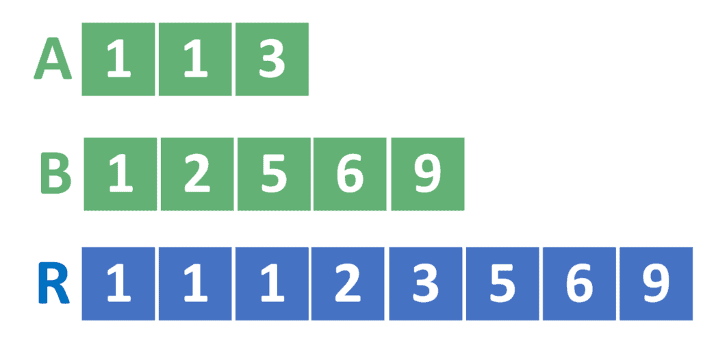
From the example, we can see that the array $A$ has $3$ elements, while the array $B$ has $5$ elements. Therefore, the resulting array $R$ has $3+5=8$ elements.

Also, the resulting array $\boldsymbol{R}$ contains all the elements from $\boldsymbol{A}$ and $\boldsymbol{B}$ . For example, the array $A$ contains the value $1$ twice. On the other hand, $B$ contains the value $1$ once. Hence, the array $R$ contains the value $1$ three times.

Also, the resulting array $R$ contains all the elements sorted in the ascending order, similarly to the arrays $A$ and $B$ .

Now that we reached a good understanding of the problem, let’s dive into the solutions.

3. Naive Approach

Let’s discuss the naive approach firstly. After that, we can see how to improve it.

In the naive approach, we simply add all the elements from arrays $\boldsymbol{A}$ and $\boldsymbol{B}$ to $\boldsymbol{R}$ . Then, we sort $\boldsymbol{R}$ before returning it.

Take a look at its implementation:

algorithm naiveMerge(A, B):
    // INPUT
    //   A = The first array
    //   B = The second array
    //   n = the size of A
    //   m = the size of B
    // OUTPUT
    //   Returns the merged array of A and B

    R <- empty array of size n + m
    id <- 0

    for i <- 0 to n - 1:
        R[id] <- A[i]
        id <- id + 1

    for j <- 0 to m - 1:
        R[id] <- B[j]
        id <- id + 1

    sort(R)
    return R

In the beginning, we’ll declare the resulting array $R$ of size $n+m$ . This array will hold the resulting answer to the problem. Also, we’ll initialize $id$ with zero that will point to the index on which to add the next element inside $R$ .

After that, we iterate over all the values inside $A$ and add them to the resulting array $R$ . Also, we perform the same operation for all the values inside $B$ .

Finally, we sort the array $R$ and return it as the resulting answer.

The complexity of the naive approach is $\boldsymbol{O((n + m) \times log(n+m))}$ , where $n$ is the number of elements inside the first array and $m$ is the number of elements inside the second one.

The reason for the complexity is that we can perform the sorting operation in $O(n \times log(n))$ .

4. Two-Pointers Approach

Let’s improve the naive approach.

4.1. Theoretical Idea

Suppose we want to find out the first element that should be added to the resulting array $R$ . It must be the smallest element inside $A$ and $B$ .

However, since both arrays $A$ and $B$ are sorted, then the smallest element of each of them is at the beginning. Therefore, we’ll add this value to $R$ .

Now, let’s imagine that we removed this smallest value from its array, and think about the problem again. We’ll need to find the new smallest element and add it to $R$ as well.

As a result, we can find a general approach to solve this problem. We start by defining two pointers $i$ and $j$ . Initially, $i$ will point to the first element in $A$ , and $j$ will point to the first element in $B$ . In each step, we’ll add the smallest value to $\boldsymbol{R}$ and move the corresponding pointer one step forward.

Note that, since we always add the smallest value to $\boldsymbol{R}$ , the resulting array $\boldsymbol{R}$ will be sorted in the end.

Since the idea is clear now, we can jump to the implementation of this approach.

4.2. Implementation

Take a look at the implementation of the two-pointers approach:

algorithm twoPointersMerge(A, B):
    // INPUT
    //   A = The first array
    //   B = The second array
    //   n = the size of A
    //   m = the size of B
    // OUTPUT
    //   Returns the merged array of A and B

    i <- 0
    j <- 0
    R <- empty array of size n + m

    for id <- 0 to n + m - 1:
        if j >= m:
            R[id] <- A[i]
            i <- i + 1 
        else if i >= n:
            R[id] <- B[j]
            j <- j + 1
        else if A[i] <= B[j]:
            R[id] <- A[i]
            i <- i + 1
        else:
            R[id] <- B[j]
            j <- j + 1

    return R

First of all, we’ll initialize two variables $i$ and $j$ with zero. These variables will serve as the needed two pointers. Therefore, $i$ will point to the current index inside $A$ , and $j$ will point to the current index inside $B$ .

Also, we’ll declare the array $R$ that will hold the resulting answer. Note that the array $R$ must be of size $n + m$ .

Next, we’ll iterate over all the indexes inside the resulting array $R$ . For each index, we’ll store the minimum value among $A[i]$ and $B[j]$ and move the corresponding pointer.

Nevertheless, we mustn’t forget about the case when either $i$ or $j$ reaches the end of their arrays. In this case, we must store the value from the other array and move its pointer.

Finally, we return the resulting array $R$ .

The complexity of the two-pointers approach is $\boldsymbol{O(n+m)}$ , where $n$ is the number of elements inside the first array and $m$ is the number of elements inside the second one.

5. Comparison

In the general case, the two-pointers approach has the lowest time complexity. However, there’s one case where the naive approach can be implemented with a complexity equal to the one of the two-pointers approach.

If all the elements inside $\boldsymbol{A}$ and $\boldsymbol{B}$ are relatively small, then we can sort the resulting array $\boldsymbol{R}$ using the counting sort technique. In this case, the counting sort has a complexity of $O(n + MaxValue)$ , where $n$ is the number of elements inside the array, and $MaxValue$ is the maximum number inside it.

Therefore, the complexity of the naive approach becomes $\boldsymbol{O(n + m + MaxValue)}$ , where $n$ is the number of elements inside the first array, $m$ is the number of elements inside the second array, and $MaxValue$ is the maximum value inside both arrays.

As a result, if $\boldsymbol{O(n + m) \geq O(MaxValue)}$ , then the complexity of the naive approach becomes $\boldsymbol{O(n + m)}$ .

Note that this complexity is similar to the complexity of the two-pointers approach. We can’t obtain a better complexity because the resulting array $R$ has a size of $n + m$ . Hence, in the best case, we still need to iterate over its elements and fill them one by one without performing any more operations.

6. Conclusion

In this tutorial, we discussed the problem of merging two sorted arrays into a resulting sorted array.

In the beginning, we discussed the problem with an example.

After that, we provided two approaches to solve the problem. The first approach was the naive one, while the second one was the two-pointers approach.

Finally, we presented a comparison between both approaches and provided the case in which both the naive and the two-pointers approaches reach the same complexity.

Full Archive

About Baeldung

Core Concepts

Operating Systems

Artificial Intelligence

Graph Theory

Latex