Finding Maximum Size Square in a Matrix Filled With Ones

1. Overview

In this tutorial, we’ll discuss finding the maximum square size filled with ones in a matrix that contains only zeros and ones.

Firstly, we’ll define the problem. Then we’ll give an example to explain it.

After that, we’ll present four different approaches to solving this problem.

2. Defining the Problem

We’re given a binary matrix $G$ of size $N \times M$ (containing $N$ rows and $M$ columns). Each cell of the matrix has a value equal to either zero or one. We’re asked to find the maximum side length of a sub-matrix that’s full of ones.

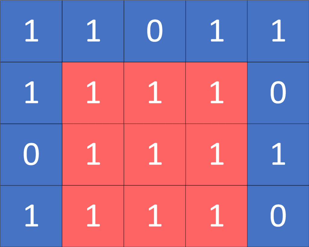
Let’s take a look at the following example for a better understanding:

we’ll represent the sub-matrix as two tuples $(x_1, y_1)$ and $(x_2, y_2)$ , which represent the position of the top-left corner and the bottom-right corner respectively.

As we can see, the sub-matrix $(2, 2)$ and $(4, 4)$ is the biggest square sub-matrix which is full of ones. It has a size equal to $3 \times 3$ , so the answer for the given example is $3$ , which represents the length of the square’s side.

3. Brute Force Approach

3.1. Main Idea

The idea in this approach is to loop over all the cells of the given matrix. For each cell, we fix it as the top-left corner and check every possible square length.

For each length, we get the bottom-right corner by adding the $length - 1$ to the coordinates of the top-left corner $(i, j)$ , which represents the current fixed cell. To check whether the current square is full of ones, we’ll iterate over all the cells of this sub-matrix and check if they’re equal to one.

In the end, if the current square is valid, we’ll maximize our answer with the current length to get the length of the maximum square full of ones.

3.2. Checking a Full Square

First, let’s implement the function that will check whether a given square matrix is filled with ones:

We iterate over each cell in the sub-matrix. If the value of the current cell is equal to zero, then we return $false$ .

Otherwise, if we reach the end and don’t find any zeros, that means the sub-matrix is full of ones. As a result, we return $true$ .

3.3. Algorithm

Let’s take a look at the implementation of the algorithm:

Initially, we declare $answer$ , which will store the answer for our problem. Then, we iterate over each cell of the given matrix and fix it as the top-left corner of the square sub-matrix.

Next, we try to check every possible length. If the current length generates a square that doesn’t fit in the matrix, we break out of the loop.

Otherwise, we check if the square sub-matrix that has top-left corner $(i, j)$ and bottom-right corner $(i + len - 1, j + len - 1)$ is full of ones. If so, that means there’s a square with a side length equal to $len$ . So, we maximize the answer to equal the maximum value between the previous answer and the current length.

Finally, the $answer$ will have the length of the maximum square that’s full of ones.

3.4. Complexity

The complexity of this algorithm is $\boldsymbol{O(N^{2} \times M^{2} \times L)}$ , where $N$ is the number of rows, $M$ is the number of columns, and $L$ is the maximum possible length of a square side which is in the worst-case equal to $Min(N, M)$ .

The reason behind this complexity is that we’ll iterate over each cell once with complexity equal to $O(N.M)$ . On the other hand, for each cell, we try every possible length with complexity that is equal to $O(L)$ .

In addition, for every length, we check if the square is full of ones or not, which has a complexity equal to $O(N.M)$ .

That leaves us with total complexity equal to $O(N^{2} \times M^{2} \times L)$ .

4. Dynamic Programming Optimization

4.1. Main Idea

In this approach, we’ll use the same idea as the previous approach. However, we’ll optimize the $isFull$ function and make it run in $O(1)$ complexity instead of $O(N \times M)$ .

We’ll use the 2D prefix sum technique, a dynamic programming optimization, to get the sum of sub-matrix in constant time complexity. The main idea in this technique is to create a $\boldsymbol{prefix}$ matrix which, inside $\boldsymbol{prefix[i][j]}$ , stores the sum of all the elements in the sub-matrix (1, 1), (i, j).

The formula to build this matrix is:

$\boldsymbol{Prefix[i][j] = Matrix[i][j] + Prefix[i][j - 1] + Prefix[i - 1][j] - Prefix[i - 1][j - 1]}$

The sum of the sub-matrix (1, 1), (i, j) can be obtained by taking the sum of sub-matrices (1, 1), (i, j – 1) and (1, 1), (i – 1, j). However, in this case, we have added the sum of (1, 1), (i – 1, j – 1) twice. Thus, we delete it from the answer. Also, we didn’t include the current cell (i, j), so we add it to the prefix value.

If we want to get the sum of a specific sub-matrix $(x_1, y_1)$ , $(x_2, y_2)$ , we’ll get the sum at the bottom-right corner $prefix[x_2][y_2]$ .

Then, we’ll subtract $prefix[x_2][y_1 - 1]$ which corresponds to the sum of the sub-matrix $(1, 1)$ , $(x_2, y_1 - 1)$ . Also, we’ll subtract $prefix[x_1 - 1][y_2]$ which represents the sum of the sub-matrix $(1, 1)$ , $(x_1 - 1, y_2)$ .

Finally, we add $prefix[x_1 - 1][y_1 - 1]$ which is the sum of the sub-matrix $(1, 1)$ , $(x_1 - 1, y_1 - 1)$ because we deleted this sub-matrix twice when we removed the previous two sub-matrices.

Let’s take the following example:

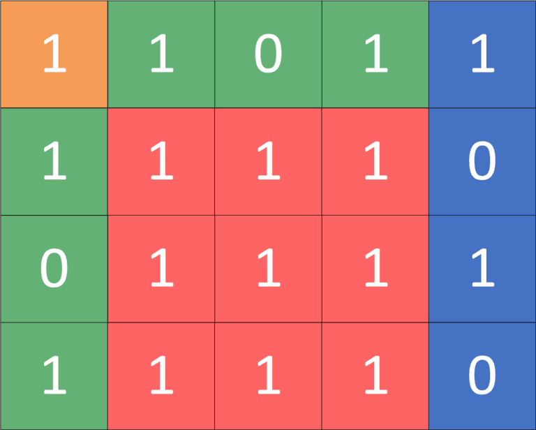
The sum of the sub-matrix (2, 2), (4, 4) can be calculated by taking the following 2D prefix values:

$sum = prefix[4][4] - prefix[4][1] - prefix[1][4] + prefix[1][1]$

4.2. Algorithm

Let’s take a look at the enhanced implementation of the $isFull$ function:

The $isFull$ function will take the top-left and the bottom-right corners as parameters. Next, we’ll calculate the area of the sub-matrix, which represents the number of cells in the sub-matrix.

After that, we’ll use the 2D prefix sum technique to get the sum of the elements in the sub-matrix, which represents the number of ones in the sub-matrix.

Finally, if the value of $sum$ is equal to the value of $area$ (number of ones equal to the number of cells), that means the given sub-matrix is full of ones. Otherwise, it’s not.

4.3. Complexity

The complexity of this algorithm is $\boldsymbol{O(N \times M \times L)}$ , where $N$ is the number of rows, $M$ is the number of columns, and $L$ is the maximum possible length of a square side which is in the worst-case equal to $Min(N, M)$ .

The reason behind this complexity is the same as the previous approach, but instead of checking if a sub-matrix is full of one in $O(N.M)$ complexity, we did it in constant time $O(1)$ .

In addition, before starting our algorithm, we’ll calculate the values of $prefix$ array, but this will have a complexity equal to $\boldsymbol{O(N \times M)}$ , which is less than the complexity of the algorithm itself.

5. Binary Search Approach

5.1. Main Idea

In this approach, we’ll use the binary search algorithm to find the maximum valid length in $\boldsymbol{O(Log_2(L))}$ .

The reason why binary search works here is that, while we iterate over the top-left corner, if there’s a square full of ones of size $L$ , that means all the squares of sizes $[1, 2, 3, ..., L]$ are also filled with ones. The reason is that the square of size $L$ is a sub-matrix of the square of size $L + 1$ .

On the other hand, if there’s a square that isn’t filled with ones of size $L$ , that means all the squares of size $[L, L + 1, ....]$ are also not filled with ones.

5.2. Algorithm

Let’s take a look at the implementation:

Initially, we declare $answer$ , which will store the answer for our problem. Then, we iterate over each cell of the given matrix and fix it as the top-left corner of the square sub-matrix.

Next, we’ll find the maximum valid length using binary search. During the binary search algorithm, if the current length is valid (gives us a square full of ones), then we’ll try to maximize the $answer$ and look for a bigger length. Otherwise, the current length is not valid, and we’ll try to find a smaller length that gives us a square full of ones.

Finally, the $answer$ will have the length of the maximum square that’s full of ones.

5.3. Complexity

The complexity of this algorithm is $\boldsymbol{O(N \times M \times Log_2(L))}$ , where $N$ is the number of rows, $M$ is the number of columns, and $L$ is the maximum possible length of a square side which is in the worst-case equal to $Min(N, M)$ .

The reason behind this complexity is the same as the previous approach, where we enhanced the $isFull$ function. Still, instead of looping over all the possible lengths, we found the perfect length using binary search technique in complexity $O(Log_2(L))$ , instead of $O(L)$ .

6. Two Pointers Approach

6.1. Main Idea

The main idea here is that there’s no need to repeat the search for a perfect length over and over again for each cell.

Instead, when we find a valid length $\boldsymbol{L}$ , we don’t have to check lengths $\boldsymbol{[1, 2, 3, .., L]}$ again since we already have a square full of ones of length $\boldsymbol{L}$ . Now, we’ll just be looking for a bigger square full of ones.

6.2. Algorithm

Let’s take a look at the implementation:

Initially, we declare $len$ , which will represent the maximum length we have at this moment. Also, it’ll be the answer to our problem.

Then, we iterate over each cell of the given matrix and fix it as the top-left corner of the square sub-matrix. Next, as long as we have a square full of ones of the current length, and we didn’t exceed the boundaries of the matrix, we increase the $len$ to find a bigger square.

Finally, the $len$ value will have the length of the maximum square that’s full of ones.

6.3. Complexity

The complexity of this algorithm is $\boldsymbol{O(N \times M + L)}$ , where $N$ is the number of rows, $M$ is the number of columns, and $L$ is the maximum possible length of a square side which is in the worst-case equal to $Min(N, M)$ .

The reason behind this complexity is that we iterate over each cell once in the complexity of $O(N \times M)$ .

In addition, we don’t reduce the value of $len$ . Instead, to find the perfect length, we iterate over each length at most once since when we find a valid length $L$ , we don’t recheck all the previous lengths.

7. Conclusion

In this article, we presented the problem of finding the maximum square that’s full of ones.

First, we provided an example to explain the problem. Then, we gave four different approaches to solving it.

Finally, we walked through their implementations, with each approach having a better time complexity than the previous one.

Full Archive

About Baeldung

Core Concepts

Operating Systems

Artificial Intelligence

Graph Theory

Latex