

Learn through the super-clean Baeldung Pro experience:
>> Membership and Baeldung Pro.
No ads, dark-mode and 6 months free of IntelliJ Idea Ultimate to start with.
Last updated: March 18, 2024
Learn through the super-clean Baeldung Pro experience:
>> Membership and Baeldung Pro.
No ads, dark-mode and 6 months free of IntelliJ Idea Ultimate to start with.
In this tutorial, we’ll show how to multiply a matrix chain using dynamic programming. This problem frequently arises in image processing and computer graphics, e.g., animations and projections.
Let’s start with an example. We have four matrices:  and
and  . Their shapes are
  ,
,  ,
,  , and
, and  , respectively.
Since each matrix’s number of columns corresponds to the next one’s number of rows, their product  is defined.
We can calculate it sequentially. First, we multiply  and
and  to get an intermediate
  -matrix
  . Then, we multiply with
  and get a
  -matrix
  . Finally, we get the result by multiplying with :
![\[\overbrace{(\underbrace{\text(A \times B)}_{M_1} \times C)}^{M_2} \times D\]](/wp-content/ql-cache/quicklatex.com-f79b2fc3a5fe83a589cd66ad4295e5fc_l3.svg "Rendered by QuickLaTeX.com")
How many operations do we perform this way?
To multiply two matrices  and
and  of shapes
  and
and  , we must compute
  elements. For each, we perform
  scalar multiplications and
  additions. So, the total number of operations,
  , is
, is  .
.
In our example:
![\[\begin{aligned} cost(A \times B) & = 4 \cdot 3 \cdot (2 \cdot 5 - 1) = 108 \\ cost(M_1 \times C) &= 4 \cdot 10 \cdot (2 \cdot 3 - 1) = 200 \\ cost(M_2 \times D) &= 4 \cdot 2 \cdot (2 \cdot 10 - 1) = 152 \end{aligned}\]](/wp-content/ql-cache/quicklatex.com-61923112ea6197b47e691945d9dbf289_l3.svg "Rendered by QuickLaTeX.com")
That’s 460 operations. However, since matrix multiplication is associative, we can compute the chain in a different order:
![\[A \times \overbrace{(B \times \underbrace{(C \times D)}_{M_1'})}^{M_2'}\]](/wp-content/ql-cache/quicklatex.com-fae250a5701c636833850c29834565ff_l3.svg "Rendered by QuickLaTeX.com")
This multiplication order involves 236 operations:
![\[\begin{aligned} cost(C \times D) & = 3 \cdot 2 \cdot (2 \cdot 10 - 1) = 114 \\ cost(B \times M_1') &= 5 \cdot 2 \cdot (2 \cdot 3 - 1) = 50 \\ cost(A \times M_2') &= 4 \cdot 2 \cdot (2 \cdot 5 - 1) = 72 \end{aligned}\]](/wp-content/ql-cache/quicklatex.com-678057209da7e27e3c9e8d1a4ffbfb6a_l3.svg "Rendered by QuickLaTeX.com")
The reduction is almost 50%.
So, in problems of this type, we have  matrices
  of the shapes
  such that
  for all
  .
.
The goal is to find the multiplication order that minimizes  , the number of scalar multiplications and additions in computing the product
  .
.
We can use dynamic programming to do this. So, let’s start with the recursive relation.
Let  (where
  ). No matter how we order multiplications, the final product will always result from multiplying two matrices.
So, we compute  by splitting it into the “left” and “right” products
  (of shape
  ) and
) and  (of shape
  ):
):
![\[(A_i \times \ldots \times A_k ) \times ( A_{k+1} \times \ldots \times A_j)\]](/wp-content/ql-cache/quicklatex.com-fded6dcc56648fcdad00858718032d5a_l3.svg "Rendered by QuickLaTeX.com")
The choice of  determines the cost:
![\[cost(i, k) + cosr(k+1, j) + p_i q_j (2 p_{k+1} - 1)\]](/wp-content/ql-cache/quicklatex.com-2b45fe6c7883e42b6ddc34a41075a71b_l3.svg "Rendered by QuickLaTeX.com")
Therefore, we should choose the that minimizes the number of operations:
![\[cost(i, j) = \begin{cases} \min_{k=i}^{j-1} \left\{cost(i, k) + cost(k+1, j) + p_i q_j (2 p_{k+1} - 1)\right\}, & j > i \\ 0, & j=i \end{cases}\]](/wp-content/ql-cache/quicklatex.com-88928b9930506e61c613a84609761da7_l3.svg "Rendered by QuickLaTeX.com")
The base case is  , and its cost is zero because we don’t perform any operation to compute
  .
.
Let’s check out the tabular approach to computing  .
.
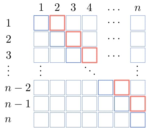
In this method, we start from the base cases and work up to one diagonal at a time. So, after the base cases on the main diagonal, we compute the costs  for of multiplying pairs:
Then, we compute the  for
for  :
:
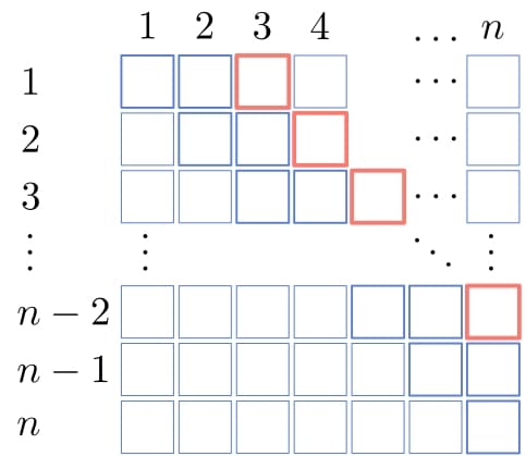
Continuing this way, we calculate in the end:
We keep track of the splitting indices by storing them in a separate data structure  as we compute the costs.
We can use  matrices for
  and , but half of the reserved space will be unused. Another option is to use a hash map.
Let’s apply these algorithms to our initial example with matrices and of shapes , , , and , respectively.
First, we set the costs on the main diagonal to zero. Then, we compute the costs of  ,
,  , and
, and  .
.
There will be only one way to split each pair. For example:
![\[cost(A \times B) = cost(A) + cost(B) + 4 \cdot 3 \cdot (2 \cdot 5 - 1) = 0 +0 + 12 \cdot 9 = 108\]](/wp-content/ql-cache/quicklatex.com-83e0560c955ca6f5e4850f3395619ae1_l3.svg "Rendered by QuickLaTeX.com")
The same goes for and :
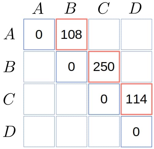
We used matrix names instead of indices for readability.
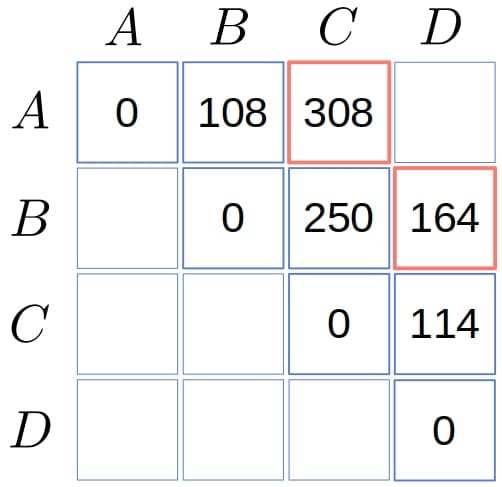
Now, we focus on  and
and  :
:
![\[\begin{aligned} cost(A \times B \times C) &= \min \begin{Bmatrix} cost(A) + cost(B \times C) + 4 \cdot 10 \cdot (2 \cdot 5 - 1) = 0 +250+40\cdot 9 = 610 \\ cost(A \times B) + cost(C) + 4 \cdot 10 \cdot (2 \cdot 3 - 1) = 108 +0 + 40 \cdot 5 = 308 \end{Bmatrix} = 308 \\ cost(B \times C \times D) &= \min \begin{Bmatrix} cost(B) + cost(C \times D) + 5 \cdot 2 \cdot (2 \cdot 10 - 1) = 0 +250+10\cdot 19 = 440 \\ cost(B \times C) + cost(D) + 5 \cdot 2 \cdot (2 \cdot 3 - 1) = 114 +0 + 10 \cdot 5 = 164 \end{Bmatrix} = 164 \end{aligned}\]](/wp-content/ql-cache/quicklatex.com-ff9260f9fa26a011c60c56f55cbb15d1_l3.svg "Rendered by QuickLaTeX.com")
So:
Finally, we compute  :
:
![\[cost(A, B, C, D) = \min \begin{Bmatrix} cost(A) + cost(B \times C \times D) + 72 =236\\ cost(A \times B) + cost(C \times D) + 40 = 398\\ cost(A \times B \times C) + cost(D) + 152 =460 \end{Bmatrix} = 236\]](/wp-content/ql-cache/quicklatex.com-5de5b2b236ed3dc1b305b0e0122dcf99_l3.svg "Rendered by QuickLaTeX.com")
A way to reconstruct the solution is to follow the indices in  recursively.
If ![T[i, j]=k](/wp-content/ql-cache/quicklatex.com-e785f33f4c2f609d98054a4dcd3de7aa_l3.svg "Rendered by QuickLaTeX.com") , where
, where  , that means that
  should be computed as
  . So, we need
 ![T[i, k]](/wp-content/ql-cache/quicklatex.com-8342ffe73d92dc7b13ea2c7c707d8575_l3.svg "Rendered by QuickLaTeX.com") and
and ![T[k+1, j]](/wp-content/ql-cache/quicklatex.com-213a539f5f00e34aeb5410a63772b695_l3.svg "Rendered by QuickLaTeX.com") to split
to split  and optimally:
The result of  is the solution for the entire input chain
  .
.
In our example, is a  matrix with the empty lower triangle:
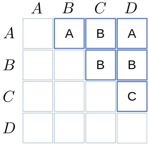
Since ![T[A, D] = A](/wp-content/ql-cache/quicklatex.com-71b66477a1b9ab30bcf77e11f82ca645_l3.svg "Rendered by QuickLaTeX.com") , the first split comes after , so we have:
, the first split comes after , so we have:
![\[A \times ( B \times C \times D)\]](/wp-content/ql-cache/quicklatex.com-4f697b2d632c277eb6072c8aacc040f8_l3.svg "Rendered by QuickLaTeX.com")
Since the left product is a single matrix, we focus on the right one. ![T[B, D] = B](/wp-content/ql-cache/quicklatex.com-59f065a3e637093621c03e668de441db_l3.svg "Rendered by QuickLaTeX.com") , so we get:
, so we get:
![\[A \times \left( B \times (C \times D) \right)\]](/wp-content/ql-cache/quicklatex.com-fc2958beee884eaeffd33a7b8a92a3a1_l3.svg "Rendered by QuickLaTeX.com")
Memoization is another approach. It computes  recursively following its definition. However, it avoids repeated calculations by memorizing the intermediate results:
For each pair  , we first check in
  if we’ve already computed
  . If so, we return
 ![memory[i, j]](/wp-content/ql-cache/quicklatex.com-6bbb8698ef735c9b3fdb61bff868e9ee_l3.svg "Rendered by QuickLaTeX.com") . Otherwise, we calculate .
. Otherwise, we calculate .
This approach is usually easier to implement than the tabular method. However, the excessive depth of the recursion tree for large can cause stack overflow.
In this article, we showed how to multiply a chain of matrices using dynamic programming.
The main difference between the tabular approach and memoization is the order in which the sub-problems are solved. The former is a bottom-up iterative approach that starts from the base cases, whereas the latter is a top-down recursive approach.


