Median of a Matrix With Sorted Rows | Baeldung on Computer Science

1. Overview

In this tutorial, we’ll talk about the problem of finding the median of a matrix with sorted rows.

First, we’ll define the problem and provide an example to explain it. Then, we’ll present two approaches to solve this problem and work through their implementations and time complexity.

2. Defining the Problem

Suppose we have a matrix $M$ of $R$ sorted rows and $C$ columns. We were asked to get the median of that given matrix $M$ . (Recall the median is the element that’s located in the middle of a sorted list).

Let’s take a look at the following example for better understanding, given a matrix $M$ with sorted rows:

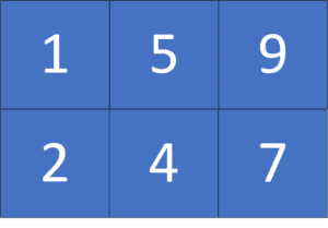
As we can see, the median here is $5$ , since if we put all the elements of the matrix $M$ in a sorted list $[1, 2, 4, 5, 7, 9]$ , then the element that is located at the middle:

$\lfloor \frac {list\_ size}{2} \rfloor = 5$

3. Naive Approach

3.1. Main Idea

The main idea of this approach is to put all the elements of the given matrix in a list, then sort it and get the middle element.

Suppose we have a matrix of $R$ rows and $C$ columns. First, we’ll iterate over it row by row. Then, for each row, we’ll insert all its elements in the predefined list $L$ , which will store all the elements of the given matrix.

Second, after having all the elements in the list $L$ , we’ll sort this list using any sorting algorithm.

Finally, the median of the given matrix is the element located at the index:

$\lfloor \frac{R \times C}{2} \rfloor$

3.2. Algorithm

Let’s take a look at the implementation of the algorithm:

Initially, we have the $Median$ function that will return the median of the given matrix $M$ . The function will have one parameter: the given matrix $M$ .

First, we declare an empty list $L$ . Then, we iterate over all the elements of the given matrix $M$ , and append them to the list $L$ .

Second, we sort the list $L$ and get the index of the middle element of the list $L$ .

Finally, we return the given matrix median, $L[ median\_ pos ]$ .

3.3. Complexity

The time complexity of the previous approach is $\mathbf{O(R \times C \times Log_2(R \times C))}$ , where $R$ is the number of rows of the given matrix $M$ , and $C$ is the number of columns. The reason behind this complexity is that we’re sorting a list of length $R \times C$ , which equals the number of elements in the given matrix.

The space complexity here is $\mathbf{O(R \times C)}$ . The reason behind this complexity is that we’re storing all the elements of the given matrix in an additional list $L$ .

4. Binary Search

4.1. Main Idea

The idea of this approach is that we’ll do a binary search on the value of the median.

Initially, we’ll do a binary search on the median value. The check of this binary search will be to count the number of elements smaller than or equal to the value we’re checking. If the count of these elements is greater than half of the matrix’s elements, then this value could be the median of the given matrix $M$ . Otherwise, we want to try more significant values.

In the end, we’ll have the element located in the middle if we sort all the elements of the given matrix.

4.2. Smaller or Equal Values

First of all, let’s take a look at the following algorithm to calculate the number of elements smaller than or equal to a specific value in the given matrix $M$ :

The function will have two parameters. The first one is $M$ representing the given matrix, while the second one is $X$ , which is the value we are checking.

First, we declare $count$ , which will store the count of elements smaller than or equal to $X$ . Next, we iterate over the rows of the given matrix $M$ . Since the rows are sorted, then for each row, we can do a binary search to find the first position that has an element greater than $\mathbf{X}$ .

Second, we’ll increase the $count$ by $pos$ since it is also the number of elements smaller than or equals $X$ in the current row.

Finally, we return $count$ , which is the number of elements smaller than or equal to $X$ in the given matrix $M$ .

4.3. Algorithm

Let’s take a look at the implementation of the algorithm for finding the median element:

Initially, we have the $Median$ function the same as the previous approach.

First, we declare $answer$ , which will store the median of the given matrix. Then, we declare the boundary of the binary search, where $low$ would be the minimum value possible, and $high$ is the maximum.

Second, we’ll get the number of elements smaller than or equal to the $mid$ . If their count is greater than or equal to the expected position of the median $\lfloor \frac{R \times C}{2} \rfloor$ , then the current $mid$ could be our median. Therefore, we update the $answer$ value and try to look for a smaller median. Otherwise, the current $mid$ is not valid, and we try to look for a bigger median.

Finally, we return $answer$ , which will be the median of the given matrix $M$ .

4.4. Complexity

The time complexity of the previous approach is $\mathbf{O(32 \times R \times Log_2(C))}$ , where $R$ is the number of rows of the given matrix $M$ , and $C$ is the number of columns. The reason behind this complexity is that we’re doing a binary search on the median value, so the logarithm of the length of the maximum range of integer values would be $32$ . Then, for each potential median, we’re checking the number of elements less than or equal to it using a binary search algorithm with complexity $O(R \times Log_2(C))$ .

The space complexity here is $\mathbf{O(1)}$ because we store the value of the median.

5. Conclusion

In this article, we discussed the problem of finding the median of a matrix with sorted rows. We defined the problem and provided an example to explain it. Finally, we provided two approaches to solve it and walked through their implementations and time complexity.

Full Archive

About Baeldung

Core Concepts

Operating Systems

Artificial Intelligence

Graph Theory

Latex