Learn through the super-clean Baeldung Pro experience:
>> Membership and Baeldung Pro.
No ads, dark-mode and 6 months free of IntelliJ Idea Ultimate to start with.
Last updated: June 13, 2023

Learn through the super-clean Baeldung Pro experience:
>> Membership and Baeldung Pro.
No ads, dark-mode and 6 months free of IntelliJ Idea Ultimate to start with.
The Marching Squares algorithm is a computer graphics algorithm introduced in the 1980s that can be used for contouring. We can use the Marching Squares algorithm to draw the lines of constant:
In this tutorial, we’ll learn how the Marching Squares algorithm determines the contour from a grid of sample points of the image.
Let’s spend a brief moment understanding the mathematically precise definition of contour lines.
We have been drawing graphs of functions of one-variable such as  or implicit functions like
  for so long, that we give the matter little thought. Plotting functions of two variables is a much more difficult task.
The trick to putting together a reasonable graph of a function of two or more variables is to find a way to cut down on the dimensions involved. One way to achieve this is to draw certain special curves that lie on the surface  . These special curves, called contour curves, are obtained by intersecting the surface with horizontal planes
  for various values of the constant
  .
.
These curves in the  -plane are called the level curves of the original function
  .
.
The level curve at height of any function is the curve in  defined by the equation
  , where is a constant. In mathematical notation,
![\[\text{Level curve at height c} = \{(x,y) \in \mathbf{R}^2| f(x,y) = c\}\]](/wp-content/ql-cache/quicklatex.com-7c5914210b18eab41e047723d8ad68bf_l3.svg "Rendered by QuickLaTeX.com")
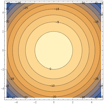
Consider the function  defined as:
![\[f(x,y)=4 - x^2 - y^2\]](/wp-content/ql-cache/quicklatex.com-3006cfe90ac12b7eb709bd257d109da0_l3.svg "Rendered by QuickLaTeX.com")
By definition, the level curve at height is:
![\[\{(x,y) | 4 - x^2 - y^2 = c\} = \{(x,y)|x^2 + y^2 = 4 - c\}\]](/wp-content/ql-cache/quicklatex.com-26bed7035ccdee148bd7c72864b512c0_l3.svg "Rendered by QuickLaTeX.com")
Thus, we see that the level curves for  are circles centered at the origin of radius
  . They are summarized in the table below:
|
 |
|---|---|
 |
 |
 |
 |
 |
 |
 |
 |
 |
 |
 |
 |
The family of level curves, the “topographic map” of the surface  is shown in the figure below:
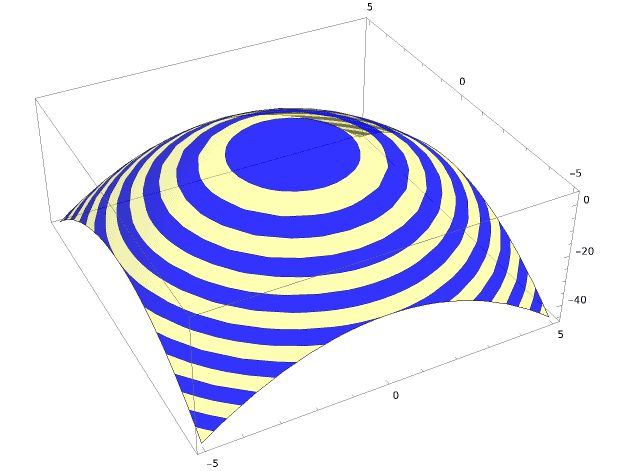
If we stack all level curves together, we can get a feeling for the complete graph of  . It’s a surface that looks like an inverted dish and is called a paraboloid:
For our discussion, we require the output contour to possess the following properties:
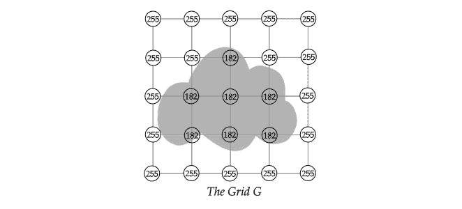
Consider the simplistic image of a cloud given below. We are interested to trace the contours of the cloud:

For simplicity, let’s assume that the image of a cloud is represented by a square matrix  of
of  pixels. Each pixel value
  represents a single sample of light, carrying brightness information. It ranges between and
  . Black is represented by and white by .
We divide the entire image domain  into
into  squares. Each square has dimensions by
  . We sample the image at each of the
  grid points:
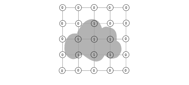
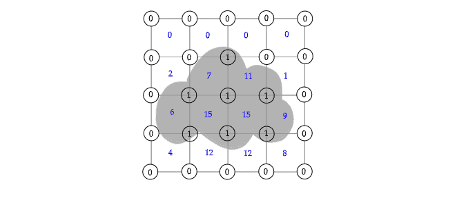
Next, we iterate through the grid  to determine the vertex state in comparison to an iso-value
  . Each grid vertex is now assigned a binary state ( or
  ). An iso-value
  serves as a threshold for determining the vertex state. Suppose we choose
  as the threshold. The vertex state is determined as follows:
 – Pixel value less than the iso-value
  – Pixel value greater than the iso-value
 The resulting binary grid  , thus obtained is:
Next, a subgrid can be associated with a configuration. We iterate through . At each sub-grid, we form a binary code based on the vertex value by iterating clockwise from the top-left corner to the bottom-left corner.
For example, if a given subgrid has four corners:

its binary code is said to be  . The equivalent of the binary code in the decimal number system is called the configuration of the sub-grid. In the above example, the sub-grid has the configuration
  Thus, we have a configuration associated with each sub-grid as follows:
Imagine a single square with the contours of an object cutting through this square. That is, the square does not lie wholly in the interior or exterior of the object. A square has edges and for each edge, we have  possible choices – either the contour(boundary) intersects this edge, or it does not. This results in
  possible configurations.
The configuration of each sub-grid is matched with one entry in the contours lookup table below:
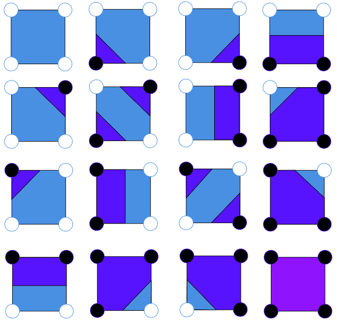
The contours lookup table is intuitive. As mentioned before, there are possible configurations.
Let’s consider the configuration  :
:

We think of the purple region as the interior of an object, and the blue region as the exterior of the object. We denote the state by a black vertex and the state by a white vertex. We define a bipolar pair to be two vertices in opposite states.
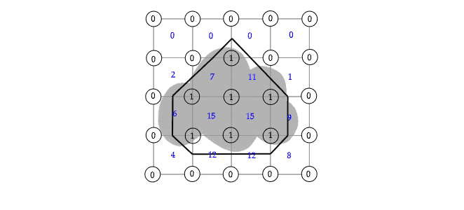
Intuitively, the contour of an object must intersect the edge of a bipolar pair. Thus, the configuration must correspond to an object whose contour intersects the top and left edges of the square. In this fashion, the contours in each sub-grid are approximated, as shown in the figure below:
The Marching Squares algorithm can be divided into two steps:
and converting them to a binary matrix . and build a set of edges  .
.Let’s see the pseudocode:
algorithm MarchingSquares(G, m, n, σ, stepX, stepY):
    // INPUT
    //    G = an m x n matrix of scalar values
    //    stepX = the sampling resolution in the x direction
    //    stepY = the sampling resolution in the y direction
    //    σ = an isovalue
    // OUTPUT
    //    γ = a set of contour lines

    F, coord, p, q <- SampleGrid(G, m, n, σ, stepX, stepY)
    γ <- March(F, coord, p, q)

return γThe input to the Marching Squares algorithm is some sample of the original matrix . The parameters  and
and  control the resolution of the sample. For example, if
  and
and  , we select the sequence of pixel-values:
![\[\begin{bmatrix} g_{0,0} & g_{0,10} & g_{0,20} & g_{0,30} & \ldots \\ g_{15,0} & g_{15,10} & g_{15,20} & g_{15,30} & \ldots\\ g_{30,0} & g_{30,10} & g_{30,20} & g_{30,30} & \ldots\\ \vdots & \vdots & \vdots & \vdots & \ddots \end{bmatrix}\]](/wp-content/ql-cache/quicklatex.com-dd744ebd2158a242965aeda3dac2433c_l3.svg "Rendered by QuickLaTeX.com")
The result of this operation should yield a matrix of size  rows and
  columns.
Each selected pixel value is compared with the iso-value and converted to a bit-value or . is used to hold the bit matrix. The actual  -coordinates of each pixel in the sample , concerning the original matrix is stored as a named tuple in a matrix
  .
.
For example, if ![G[15][20] = 100](/wp-content/ql-cache/quicklatex.com-051585a3f33dc5d08a4a5f8824d9e3d4_l3.svg "Rendered by QuickLaTeX.com") , , we would find
, , we would find ![F[1][2]=1](/wp-content/ql-cache/quicklatex.com-5d919091bae923e93ee479bec89b736b_l3.svg "Rendered by QuickLaTeX.com") ,
, ![\text{coord}[1][2]=(x=15,y=20)](/wp-content/ql-cache/quicklatex.com-22029de6df6f227db09f180317b6e5dd_l3.svg "Rendered by QuickLaTeX.com") .
.
Let’s see the pseudocode now:
algorithm SampleGrid(G, m, n, σ, stepX, stepY):
    // INPUT
    //    G = an m x n matrix of scalar values
    //    m = number of rows in the matrix G
    //    n = number of columns in the matrix G
    //    σ = an isovalue
    //    stepX = sampling resolution along the X-axis
    //    stepY = sampling resolution along the Y-axis
    // OUTPUT
    //    F = binary field
    //    coord = named tuple (x, y) indicating each pixel's position in the sample
    //    p = number of rows in the resulting matrix after sampling
    //    q = number of columns in the resulting matrix after sampling

    // Create a zero matrix to hold the binary field and xy-coordinates
    p <- m / stepX
    q <- n / stepY
    F <- zero matrix of size p x q
    coord <- zero matrix of size p x q

    // Sample the grid points
    for i <- 0 to p - 1:
        for j <- 0 to q - 1:
            if G[i * stepY, j * stepX] > σ:
                F[i, j] <- 0
            else:
                F[i, j] <- 1
            // Each entry in coord matrix is a named tuple (x, y)
            coord[i, j] <- (x = j * stepX, y = i * stepY)

    return F, coord, p, q
Next, we march the squares in the binary grid . Each square in , beginning with its top-left corner, has vertices, in clockwise order : ![F[i,j]](/wp-content/ql-cache/quicklatex.com-73500904fee397df9c8d31fd6c640bf1_l3.svg "Rendered by QuickLaTeX.com") ,
, ![F[i,j+1]](/wp-content/ql-cache/quicklatex.com-1c0530d5d5276732e89b9ff294cbadf2_l3.svg "Rendered by QuickLaTeX.com") ,
, ![F[i+1,j+1]](/wp-content/ql-cache/quicklatex.com-c14c98e2b9644824eba02ea5d28f943f_l3.svg "Rendered by QuickLaTeX.com") and
and ![F[i+1,j]](/wp-content/ql-cache/quicklatex.com-76829f2db5e4597308fe6b3728b7fb68_l3.svg "Rendered by QuickLaTeX.com") . We compute the reference value
. We compute the reference value  of each square. We also compute the mid-points of each square edge: north, east, south, and west. Finally, we determine the contour
  by searching the reference value in the contours lookup table:
algorithm March(F, Coord, p, q):
    // INPUT
    //    F = the binary field matrix
    //    Coord = the matrix of coordinates
    //    p = the number of rows in F
    //    q = the number of columns in F
    // OUTPUT
    //    γ = a set of contour lines

    γ <- an empty set

    // Compute the reference value for each grid square and lookup in the isocontour table
    for i <- 0 to p - 2:
        for j <- 0 to q - 2:
            a <- Coord[i, j]
            b <- Coord[i, j + 1]
            c <- Coord[i + 1, j + 1]
            d <- Coord[i + 1, j]

            k <- 8 * F[i, j] + 4 * F[i, j + 1] + 2 * F[i + 1, j + 1] + F[i + 1, j]

            // Compute isocontour vertex coordinates
            north <- (a.x + b.x / 2, a.y)
            east <- (b.x, (b.y + c.y) / 2)
            south <- ((d.x + c.x) / 2, d.y)
            west <- (a.x, (a.y + d.y) / 2)

            S <- LUT(k, north, east, south, west)
            γ <- γ + S

    return γ
Here’s a topographical map of the Mont Blanc region in the Swiss Alps. The Marching Squares algorithm when executed on this image produces nice contours around the mountain peaks:
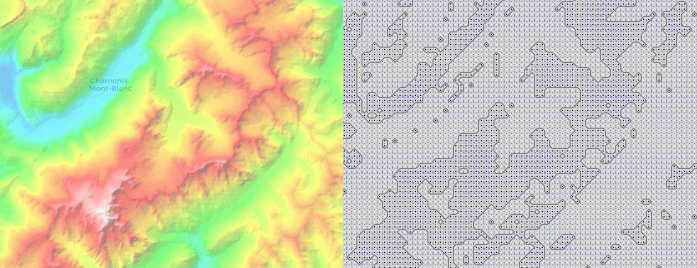
In this article, we learned about an interesting Computer Graphics algorithm called the Marching Squares. To summarize, it is based on two core ideas. First, the contours can be constructed piecewise within each grid square, without reference to other squares. Second, each isocontour segment in a grid square can be retrieved from a lookup table.