Finding the Lowest Common Ancestor of Two Nodes in a Binary Tree

1. Introduction

Binary trees have different applications in computer science and various fields. And to make use of them, we need to have a set of efficient algorithms that operate on them.

One of the common algorithms is finding the Lowest Common Ancestor (LCA) of two nodes in a binary tree, which is the topic of our tutorial this time.

2. Problem Explanation

The problem of finding the Lowest Common Ancestor is formed as follows:

Given a binary tree and two nodes, we need to find the lowest common parent of both nodes in the given binary tree. To clarify, we should recall that a tree (and binary tree as a special case) is a special case of graphs where there’s exactly one path between any two nodes.

In our post, we’re talking about the special case of a binary tree which is a tree that has a root with two connections referred to as left and right children. Then, each node also can have right or left children or both. Since we have a path between any two nodes in the binary tree, then we have a path between any node and the root node.

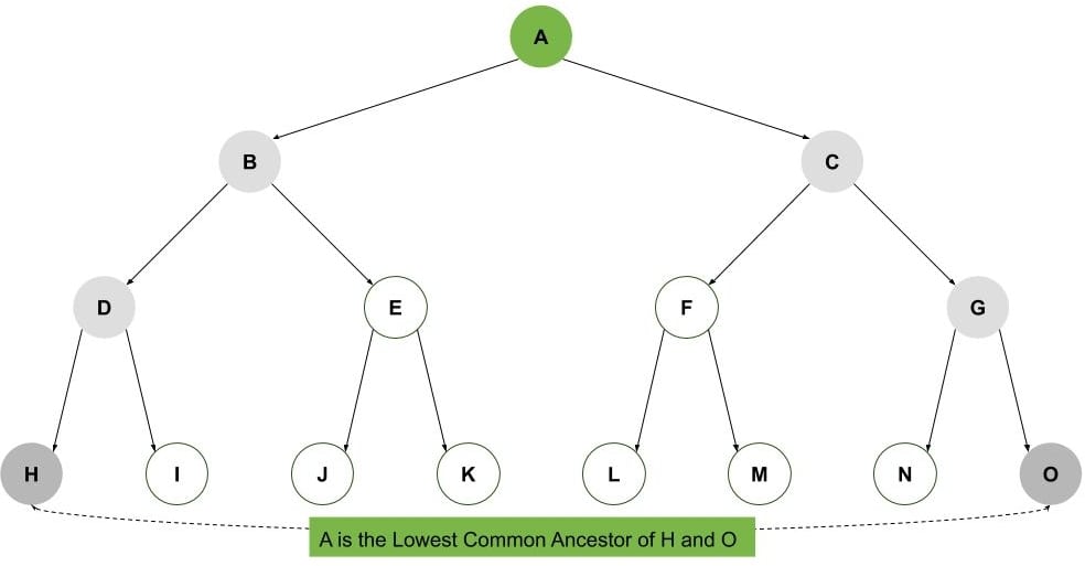
Thus, for any two nodes in a binary tree, the root is a common ancestor. Let’s see an example to elaborate on the idea. In this example, nodes ‘H’ and ‘O’ are leaf nodes and they have the root ‘A’ as a common ancestor (which happens to be the lowest common ancestor as well):

But we’re not looking for just any common ancestor for a given two nodes, we’re looking for their lowest common ancestor.

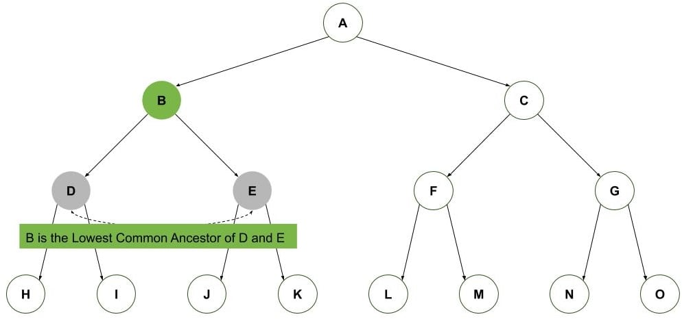
So, in the following figure, we can see that ‘B’ is the lowest common ancestor of nodes ‘D’ and ‘E’ (even though they also have a common ancestor of ‘A’):

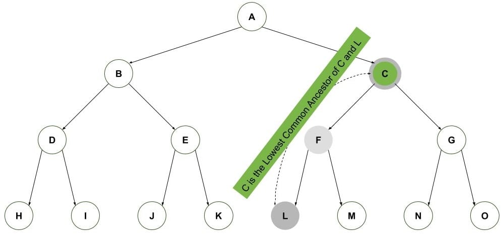
Let’s see one last example. We have two nodes where one of the nodes ‘C’ is one of the parents of the other node ‘L’. Thus, the lowest common ancestor, in this case, becomes the parent node ‘C’:

So, let’s next discuss how an algorithm we can use to find the lowest common ancestor.

3. LCA Algorithm

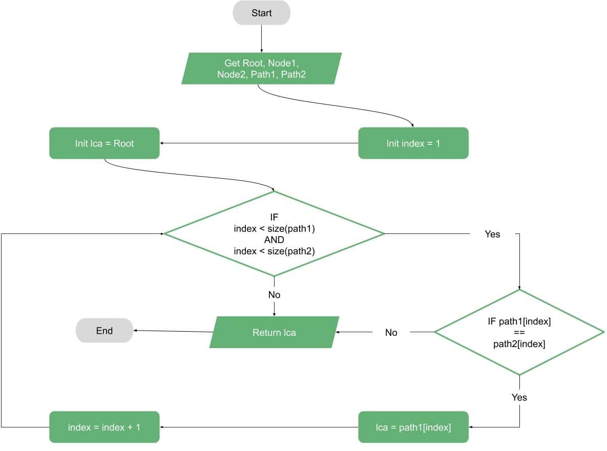
Let’s assume for the sake of simplicity that we have a function that gives the path from the root to each of the target nodes. Then, it’s an easy problem to find the lowest common ancestor by simply iterating over the two paths and finding the last common node in both paths.

Since we know that the first node in both paths is the root, we can initialize our LCA algorithm output by the root and search starting from the second index in the paths as shown:

Now, our second step is to dig deeper and define the function that finds the path from the root to any node.

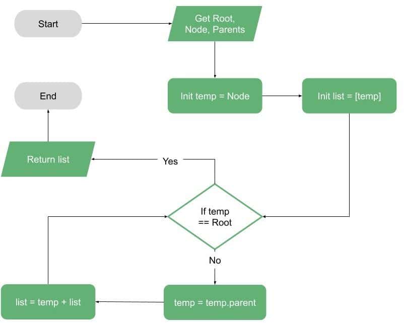
Let’s assume for the sake of simplicity one more time that we have the parents of each node in the tree given. Then, finding the path from the root to any node is a simple iteration from a node to its parent and so on until we reach the root.

Then, the path is the list of parents found along the path to the root:

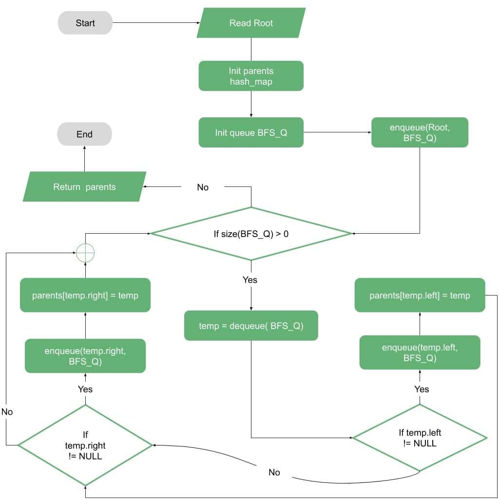
Now, to resolve our final simplification we need to find the parents for each node in the tree. Thus, we show the idea in the following flowchart which is nothing but the famous Breadth-First Search (BFS) algorithm.

One thing to remember in the BFS is saving the parents while traversing the tree. As we all know, the BFS can be implemented using an iterative method using a queue or recursive (our flowchart shows the iterative):

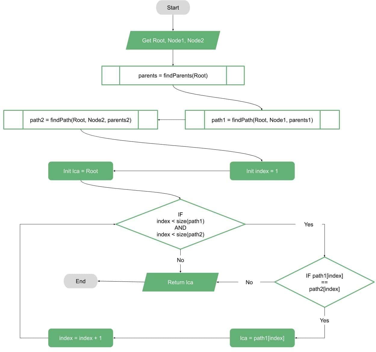
Finally, we can look at the full flowchart for finding the LCA of two nodes in a binary tree. Since the algorithm needs calls to different methods, we’ve included these parts as function calls (find parents and find path) which can be found in the previous two flowcharts:

4. Pseudocode

Now, our next step is to write simple pseudocode for the LCA algorithm.

Let’s start with the function that finds the path from the root to any node:

algorithm FindPath(Root, Node, parents):
    // INPUT
    //   Read Tree Root, Node, parents
    // OUTPUT
    //   Path from Root to Node

    temp <- Node
    path <- [temp]

    while temp != Root:
        temp <- parents[temp]
        path <- temp + path

    return path

Then, we define a function that finds the parents for each tree node (the BFS with parents saved):

algorithm FindParents(Root):
    // INPUT
    //   Read Tree Root, Node
    // OUTPUT
    //   Hash map of tree parents

    parents <- {Root: NULL}
    BFS_Q <- []

    enqueue(Root, BFS_Q)

    while size(BFS_Q) > 0:
        temp <- dequeue(BFS_Q)

        if temp.left != NULL:
            enqueue(temp.left, BFS_Q)
            parents[temp.left] <- temp

        if temp.right != NULL:
            enqueue(temp.right, BFS_Q)
            parents[temp.right] <- temp

    return parents

Finally, we define the full LCA algorithm pseudocode that uses the two previous functions:

algorithm FindLCA(Root, Node1, Node2):
    // INPUT
    //   Read Tree Root, Node1, Node2
    // OUTPUT
    //   Lowest Common Ancestor of the Two Nodes

    parents <- FindParents(Root)
    path1 <- FindPath(Root, Node1, parents)
    path2 <- FindPath(Root, Node2, parents)

    index <- 1
    lca <- Root

    while index < minimum(size(path1), size(path2)):
        if path1[index] = path2[index]:
            lca <- path1[index]
            index <- index + 1
        else:
            break

    return lca

5. Complexity

We can’t leave the LCA discussion without analyzing the complexity of our algorithm. So, let’s discuss the complexities of our LCA algorithm components:

The first component was finding the path from the root to each of the two target nodes. This is a function in the binary tree height . So, the complexity of this part is . In a balanced tree with nodes, the height approximately equals . For an unbalanced tree, it could be as bad as .

The second function is finding the parents of all nodes in the binary tree and this is mainly a Breadth-First Search, so the complexity of this part is .

Finally, the main algorithm is comparing the two paths to find the lowest common ancestor, which has the same complexity as the first part, finding the path.

And the final complexity is the summation of the three components. So, the overall time complexity is .

In the case of having the parents given with the binary tree, the complexity of the algorithm becomes . And. if we’ve got a balanced binary tree, the time complexity of the algorithm becomes .

As for the space-complexity, the algorithm requires a space of to find the parents and to save the paths. So, the overall space-complexity becomes . Also, in the case of having the parents given and the tree is balanced, we get space complexity of .

6. Conclusion

In this article, we tried to show a simple way to solve the Lowest Common Ancestor problem of two nodes in a binary tree.

We started the article with a simple introduction and explanation of the problem. Then, we explained the idea with simple flowcharts. Then, we wrote pseudocodes for the algorithm parts.

Finally, we discussed the time and space complexity analysis for the LCA algorithm.