

Yes, we're now running our only Summer Sale. All Courses are 30% off until 20th July, 2026:
Learn through the super-clean Baeldung Pro experience:
>> Membership and Baeldung Pro.
No ads, dark-mode and 6 months free of IntelliJ Idea Ultimate to start with.
1. Overview
In this tutorial, we’ll discuss the problem of finding the local minimum in a 
 x matrix.
First, we’ll define the problem and provide an example that explains it.
Second, we’ll present a naive approach and then improve it to obtain a better solution.
2. Defining the Problem
Suppose we have a matrix of size x that consists of x distinct integers. Our task is to find a local minimum in the given matrix.
Recall that a local minimum in a  matrix is the cell that has a value smaller than all its adjacent neighboring cells.
A cell has four adjacent neighboring cells if it’s inside the matrix. Furthermore, it has three adjacent neighboring cells if it’s on the border of the matrix. Finally, it has only two adjacent neighboring cells if positioned on any corner of the matrix.
Let’s check an example for better understanding. Suppose we have the following matrix of size  x:
x:
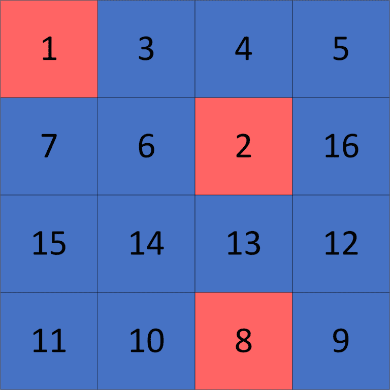
As we can see, there are three local minimum cells in our example:
 , because all of its two adjacent neighboring cells have a value greater than
  .
. , because all of its four adjacent neighbor cells have a value greater than
  .
. , because all of its three adjacent neighbor cells have a value greater than
  .
.
Therefore, the answer to our example could be any cell of these three local minimum cells.
3. Naive Approach
3.1. Main Idea
The main idea here is to always move to the smallest adjacent neighbor cell with a value smaller than the current cell value until we reach a local minimum.
To iterate over our matrix, we’ll use DFS (Depth First Search). Each time we reach a cell, we’ll check whether it’s a local minimum, which means that we’re done because we found a local minimum in the given matrix. Otherwise, we’ll move to the cell with the smallest value among all the adjacent cells that have a value smaller than the current cell value.
Eventually, this must terminate because moving to a cell with a value smaller than the current cell value cannot go on forever.
3.2. Implementation
Let’s take a look at the implementation:
algorithm FindLocalMinimumNaive(N, M):
    // INPUT
    //    N = the length of the matrix side
    //    M = the input NxN matrix
    // OUTPUT
    //    Returns a local minimum in the given matrix M

    function GetNextCell(current, M):
        x <- current.row
        y <- current.column
        value <- M[x, y]
        next_cell <- current
        if x > 1 and value > M[x - 1, y]:
            value <- M[x - 1, y]
            next_cell <- Cell(x - 1, y)
        if y > 1 and value > M[x, y - 1]:
            value <- M[x, y - 1]
            next_cell <- Cell(x, y - 1)
        if x < len(M) and value > M[x + 1, y]:
            value <- M[x + 1, y]
            next_cell <- Cell(x + 1, y)
        if y < len(M[0]) and value > M[x, y + 1]:
            value <- M[x, y + 1]
            next_cell <- Cell(x, y + 1)
        return next_cell

    function FindLocalMinimum(current):
        next_cell <- GetNextCell(current, M)
        if next_cell = current:
            return current
        else:
            return FindLocalMinimum(next_cell)
Initially, we declare the  function that will return the smallest adjacent neighbor cell with a value smaller than the current cell value. For each cell, there are four possible adjacent cells we have to check.
First, we’ll declare  and
and  values representing the current row (
 ) and the current column (
 ), respectively. Then we declare
  , which represents the value of the smallest adjacent cell. Initially, we assign the value of the current cell to it. Finally, we declare the
  , which will represent the smallest adjacent cell. To begin, it’ll be equal to the
  cell.
cell.
Next we’ll check whether the current row index is greater than , which means a cell above the one. Then we’ll check whether that cell’s value is smaller than the minimum value that we got so far. If so, we’ll update the to be equal to the cell located above the cell. We do the same process for the left, right, and down adjacent cells.
In the end, we return the that we’ll move to in the next DFS traversal.
Then we declare the  function, which returns the local minimum in the given matrix. To start, we get the that we’ll move to in the next DFS call. Second, we’ll check whether equals the cell, which means that the cell is a local minimum because it has no adjacent cell that has a value smaller than the value of the cell. Otherwise, we move to the in our DFS traversal.
3.3. Complexity
The complexity of this approach is the same as the DFS complexity, which is  , where
  is the number of cells and
  is the number of transitions. Thus, it’s
  because the number of cells is
  , while the number of transitions is a little less than
  . The reason behind this complexity is that we’ll iterate over each cell once in the worst-case scenario. Therefore, we iterate over its adjacent neighbors. In total, we iterate over each transition once as well.
4. Divide-and-Conquer Approach
4.1. Main Idea
We’ll divide the given matrix into four quadrant sub-matrices. We can guarantee that our local minimum will be inside one of these four sub-matrices. To find in which sub-matrix our local minimum exists, we’ll iterate over the  and the
  to get the cell that has the smallest value among all of the values in the and the .
After we get the cell with the smallest value, we’ll get the (smallest adjacent cell) of it. Now the sub-matrix that has the will also have the local minimum in it. This is true because if the local minimum is in another sub-matrix, it means we have to cross the or the , and that’s impossible because we’ve picked the cell that has the smallest value among all the and the cells.
Let’s take a look at the following example for better understanding:
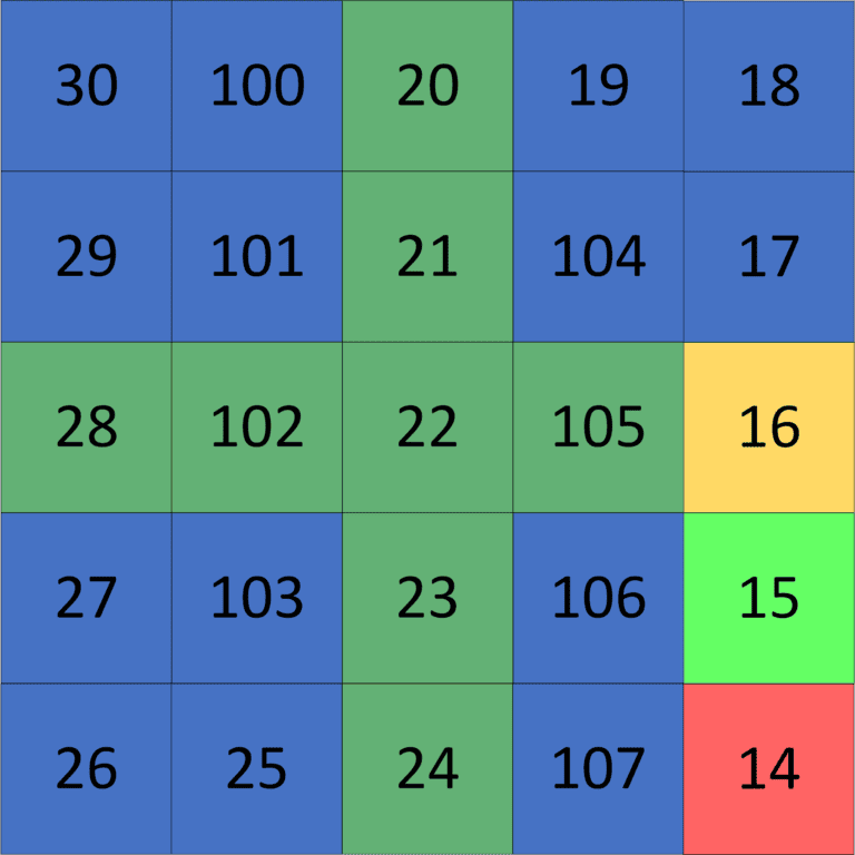
We take  , which has the smallest value among all the and the cells. Then we get the of it which is
  . So we can guarantee that the local minimum will be inside the
  sub-matrix. Therefore, we solve our problem for the sub-matrix and repeat the same process.
4.2. Implementation
Let’s take a look at the implementation:
algorithm FindLocalMinimumDivideConquer(N, M):
    // INPUT
    //    N = the length of the matrix side
    //    M = the input NxN matrix
    // OUTPUT
    //    Returns a local minimum in the given matrix M

    function FindLocalMinimum(M):
        middle_row <- len(M) / 2
        middle_column <- len(M[1]) / 2
        min_cell <- Min(GetMinInRow(middle_row, M), GetMinInColumn(middle_column, M))

        next_cell <- GetNextCell(min_cell, M)

        if next_cell = min_cell:
            return min_cell
        else if next_cell.row < middle_row:
            if next_cell.column < middle_column:
                return FindLocalMinimum(Top-Left Sub-Matrix)
            else:
                return FindLocalMinimum(Top-Right Sub-Matrix)
        else:
            if next_cell.column < middle_column:
                return FindLocalMinimum(Bottom-Left Sub-Matrix)
            else:
                return FindLocalMinimum(Bottom-Right Sub-Matrix)
Initially, we declare the function that’ll take the given matrix and return a local minimum cell in it.
Then we declare the indices of the and . After that, we declare the  , representing the cell that has the smallest value among all the cells that lay in the and . To do that, we use the
  , and
, and  functions that return the minimum value in a certain row or column, respectively.
We’ll get the of the as we did in the previous approach to know in which sub-matrix our local minimum is located.
Now we’ll check if the is equal to the . In this case, it means the is a local minimum, so we return it and finish the algorithm at this point.
However, if the  is less than the , it means that our local minimum is either in the Top-Left or Top-Right sub-matrices. Therefore, we have to check whether the
  is less than , meaning we have a local minimum in the Top-Left sub-matrix. Otherwise, it’ll be in the Top-Right sub-matrix.
Finally, we’ll check if the is greater than or equal to the , which means that our local minimum is either in the Bottom-Left or Bottom-Right sub-matrices. We check it in the same manner as we did in the previous conditions.
4.3. Complexity
The complexity here is  . Let’s examine the reason behind this complexity.
In the first call, we iterate over  cells to get the . However, in the second call, we iterate over
  cells. After that, we iterate over
  cells, and so on.
So the total number of iterations will be equal to  , which means the complexity is .
5. Conclusion
In this article, we presented the problem of finding a local minimum in a matrix. We explained the general idea and discussed two approaches.
First, we explained the naive one. Then we improved it to get the  approach, which was much faster than the first one.