LL vs. LR Parsing | Baeldung on Computer Science

1. Introduction

In this tutorial, we’ll discuss the differences between the two types of parsers that have seen wide adoption in industry and academia – LL parsers and LR parsers. We’ll contrast them using grammar theory for a deeper understanding.

2. Overview of Compilation Process

Both kinds of parsers fit into the syntax analysis phase of the compilation process. A compiler processes source code through a number of layers of abstraction, each with different inputs and outputs. The final output at the end of this pipeline is well-optimized machine code, targeted towards the architecture of the machine on which the compiler executed. As such, a parser must be both efficient in terms of runtime and powerful enough to handle the grammar in which the original source code was written.

In the classical formulation below, the lexical analyzer outputs a stream of tokens, and the syntax analyzer, of which the parser is a key component, generates a parse tree. How the parser is implemented, how the parse tree is constructed and the kind of grammars it can handle characterizes the fundamental differences between LL and LR:

3. Comparison

3.1. Parse Tree Construction

LL parsing adheres to the top-down paradigm. In other words, the parse tree is constructed starting from the root, and each node is constructed in a pre-order pattern. It can be seen as the problem of finding a suitable leftmost derivation for the input string. For example, if our production rules are $\{S \rightarrow SS, S \rightarrow a\}$ and our desired string of terminal symbols is $aaaa$ , then one possible leftmost derivation is $S => \mathbf{S}S => \mathbf{S}SSS => a\mathbf{S}SS \stackrel{*}{=}> aaaa$ .

At each step of a top-down parse, the parser determines the production rule to be applied for a given non-terminal grammar symbol $X$ . Once a production rule is chosen, it then matches terminal symbols in the body of the production rule with the input string. A grammar is then designated as $LL(k)$ if the correct production rule can be chosen by looking $k$ symbols ahead in the input. A typical value of $k$ is $1$ .

In contrast, LR parsing adheres to the bottom-up paradigm. The parse tree for an input string is constructed starting from the leaves and parsing continues upwards till it reaches the root. The goal is to reduce the input string to the start symbol $S$ of the grammar or to construct a rightmost derivation in reverse.

The parsing process consists of a series of shift and reduce-actions until we approach the start symbol. At each step, the specific substring matching the production rule body is replaced by the corresponding non-terminal symbol. Such a substring is called a handle. For e.g., given a set of production rules $\{E \rightarrow T, T \rightarrow F, T \rightarrow T * F, F \rightarrow id\}$ which represents a simple mathematical expression and the input string $id * id$ , we’d move in reverse – $\mathbf{id} * id => \mathbf{F} * id => T * \mathbf{id} => T * F => E$ . Note that $E$ is the start symbol in this case. Similar to the $LL(k)$ designation, we denote a grammar as $LR(k)$ if we can read the input by $k$ symbols ahead.

3.2. Accepted Grammars

There are certain rules for grammar to be designated as $LL$ or $LR$ . There cannot be any conflicts during the parsing process, because this would mean that the grammar is not suitable for the given parser. One example is that of a shift-reduce conflict in $LR$ parsers, where at some step, the parser cannot decisively choose between a shift and a reduce-action.

A grammar is $LL(1)$ if and only if whenever a production rule $A \rightarrow \alpha|\beta$ exists, where $\alpha$ and $\beta$ are non-terminal symbols, the following holds -:

For no terminal symbol $a$ do $\alpha$ and $\beta$ derive strings beginning with $a$ .
At most one of the two non-terminals can derive the null symbol.
If $\beta$ derives the null symbol, then $\alpha$ cannot derive any string beginning with a terminal in the $FOLLOW$ set of $A$ .

The first two conditions can be summarized as $FIRST(\alpha) \cap FIRST(\beta) = \phi$ . The last condition can be summarized as $FIRST(\alpha) \cap FOLLOW(A) = \phi$ , where $FIRST$ and $FOLLOW$ are defined in the usual way. Correspondingly, these rules can be generalized for $LL(k)$ grammars with any positive integer $k$ .

In contrast, there is a variety of parsers and corresponding grammars under the $LR(k)$ umbrella. The power of a parser is defined according to how large the subset of accepted grammar is. Among $LR$ parsers, the $SLR(1)$ parser is at the bottom of this power scale.

LR parsers make use of the $LR(0)$ state automaton, and we’ll consider item-sets within a state when defining the rules for a grammar to be accepted. For e.g., a grammar is $SLR(1)$ if it is accepted by the $SLR(1)$ parser, which happens under the following conditions -:

For each item-set, and for all items $A \rightarrow u.xv$ ( $x$ terminal) in those sets, there is no complete item $B \rightarrow w.$ in the set, where $x\ \epsilon\ FOLLOW(B)$ . This means that no shift-reduce conflict can exist.
For all pairs of complete items $A \rightarrow u.$ and $B \rightarrow v.$ , $FOLLOW(A) \cap FOLLOW(B) = \phi$ . This means that no reduce-reduce conflict can exist.

Note that a complete item is one in which the dot is at the end of the production rule, and it refers to the case where the parser can only perform a reduce-action using that production rule.

Higher-powered parsers such as the canonical $LR(1)$ and $LALR(1)$ have similar rules for the grammars they accept. Note that $LL$ grammars are a subset of $LR$ grammars, so $LL$ parsers possess less power than $LR$ parsers:

3.3. Limitations

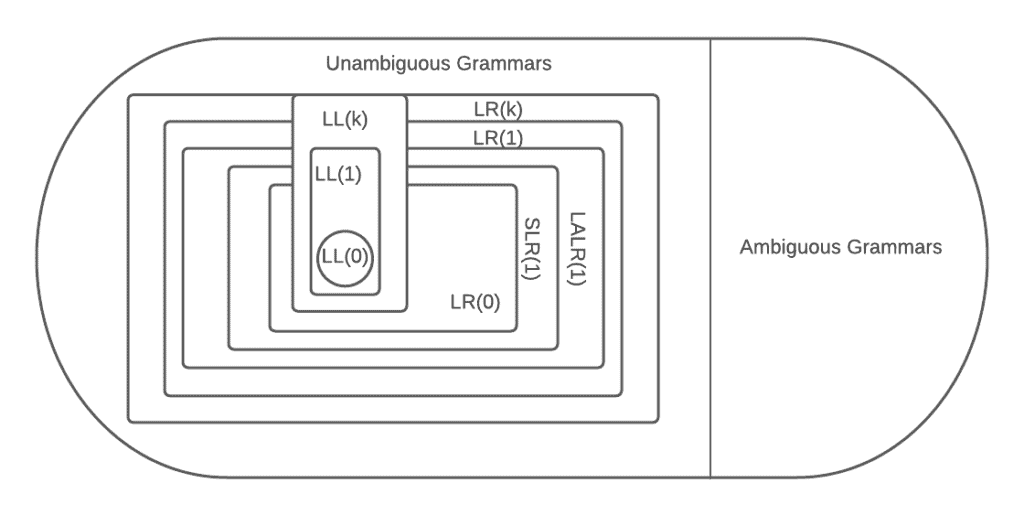
LL parsers such as the table-driven predictive parser cannot process strings from grammars that possess left-recursive production rules. Intuitively, this is because they may end up in an infinite loop while trying to process the leftmost derivation. In our earlier example of such a derivation, the rule $S \rightarrow SS$ cannot be allowed in the grammar for this reason. However, $LR$ parsers do not have this weakness and can process input strings from grammars that have left-recursive rules.

Note that among the popular top-down parsers, the recursive-descent parser is able to process strings from grammars outside the $LL$ set, but the execution is not guaranteed to terminate if the grammar is not $LL$ . In fact, even if it does terminate, it may take exponential time in the worst case. This is in contrast to the table-driven predictive parser, which cannot process strings from grammars outside the $LL$ set at all. Thus they are both considered primarily $LL$ parsers.

Both LL and LR parsers have trouble processing strings from ambiguous grammars. Ambiguity inserts conflicts in the parsing process, and so, the set of ambiguous grammars is generally considered separate from the set of $LL$ / $LR$ grammars. But while no $LL$ parser can process ambiguity, there is a type of $LR$ parser that can process a subset of $LR$ grammars known as operator grammars. This parser is suitably called an operator-precedence parser.

Ambiguity as in the traditional sense – which rule to apply next – is allowed in the operator grammar. This is because production rules are framed in a way that assigns relative precedence. The operator-precedence parser exploits these precedence rules during execution to quell ambiguity.

4. Conclusion

In summary, we’ve covered at length some of the differences between $LL$ and $LR$ parsers. We delved into grammar theory for a deeper and more fundamental understanding. In the process, we discussed several kinds of parsers.

Full Archive

About Baeldung

Core Concepts

Operating Systems

Artificial Intelligence

Graph Theory

Latex