How to Measure Sortedness? | Baeldung on Computer Science

1. Introduction

In this tutorial, we’ll discuss several ways of quantifying the extent to which an array is sorted.

2. Sortedness

We have an array $a = [a_1, a_2, \ldots, a_n]$ and want to quantify how close it is to its sorted permutation.

So, whatever we define this measure, a completely sorted array such as:

$\begin{bmatrix} 1, & 10, & 25, & 56, & 111 \end{bmatrix}$

should have a better score than a partially sorted one:

$\begin{bmatrix} 1, & 25, & 111, & 10, & 56 \end{bmatrix}$

The metric should be defined in a way that allows for comparing two partially sorted arrays and concluding which one is more sorted.

It should also apply to any data type with an ordering relation, e.g., numbers and $\geq$ or strings and lexicographic ordering. We’ll cover the general case and denote the order as $\preceq$ .

3. Inversions

An inversion in an array is a pair $\boldsymbol{(a_i, a_j)}$ whose elements are out of order:

$i < j \land a_i \not\preceq a_j$

A natural way to define sortedness is to count inversions:

$\left| \{ (i, j) \in \{1, 2,\ldots, n \}^2 \colon i < j \land a_i \not\preceq a_j \} \right|$

For example, $[1, 25, 111, 10, 56]$ contains three inversions: $(25, 10)$ , $(111, 10)$ , and $(111, 56)$ . We consider it more sorted than $[25, 1, 111, 10, 56]$ that has four inversions and less than $[1, 10, 111, 25, 56]$ with two.

By definition, the metric’s higher values correspond to less sorted arrays. So, a completely sorted array has zero inversions. An array sorted in the opposite direction has $\boldsymbol{\frac{n(n-1)}{2}}$ inversions: $n-1$ inversions containing the first element, $n-2$ inversions with the second, and down to one inversion with $a_{n-1}$ .

3.1. Scaling

We can compare any two arrays by their inversion counts, but the comparison will be fair only if they have the same number of elements. For instance, three inversions in a $10$ -element array don’t denote the same degree of sortedness as three in a $100$ -element sequence.

To consider different sizes, we can divide the count with its maximum value of $\boldsymbol{n(n-1)/2}$ . This way, we get a metric whose values are in the range $[0, 1]$ , where $0$ corresponds to a completely sorted array and 1 to a completely inverted sequence.

Let’s check out a few ways of computing this metric.

4. The Exact $\boldsymbol{O(n^2)}$ Approach

The straightforward way is to traverse the array with two loops:

We compare each $a_i$ with the elements to the right of it.

This approach is intuitive but has a quadratic time complexity. So, it isn’t practical for very large arrays.

5. The Sampling Approach

One way to avoid the performance issue is to count the inversions stochastically. That means sampling a predefined number of pairs and counting inversions among them:

When sampling, we need to ensure we don’t draw the same index twice and get $(a_i, a_i)$ as a pair to check. To see why, let’s recall that the condition $i < j$ is in the definition of an inversion, which implies that $i \neq j$ . This seems obvious, but it’s easy to overlook.

5.1. Shortcomings

In practice, this approach will be faster than the $O(n^2)$ solution but has several drawbacks:

it can return a different result each time with run it on the same array
we need to fine-tune $m$ since a value too small is likely to miss many inversions, whereas a too-large $m$ will make the execution longer
the algorithm can get stuck in a loop if it never draws different indices, which is very unlikely but still possible
we can end up checking the same pair or counting the same inversion multiple times

The first issue can be addressed by running the algorithm several times and returning the average result. Alternatively, we can use a larger $m$ if it doesn’t cause the method to run too long. Although the algorithm can run forever, it rarely happens in practice, especially with large values of $n$ and $m$ .

To fix the last drawback, we can sample the pairs without repetition.

5.2. Sampling Without Repetition

That means we should store the sampled pairs and ignore them if we draw them again:

Whenever we draw a new index pair $(i ,j)$ , we check if we considered it before. If yes, we’ll skip it. Otherwise, we’ll insert it into $memory$ to ignore it in the future.

For this approach to be efficient, the $memory$ storage should be a data structure with efficient insertions and lookups, such as a hash table. Because of the overhead, this will be slower than sampling with repetition but more accurate.

6. Merge Count

Another way is to tweak a sorting algorithm to count inversions.

Not all algorithms will be easy to modify since we aren’t supposed to count swaps done during sorting but only the inversions in the original array.

Here’s a modification of Merge Sort:

To scale the count, we divide it with $\frac{n(n-1)}{2}$ . The trick is to realize that the total number of inversions in $a$ is the sum of the counts of three types of inversions:

when $a_i$ and $a_j$ are in the left half
when $a_i$ and $a_j$ are in the right half
$a_i$ is in the left and $a_j$ in the right halves (cross-inversions)

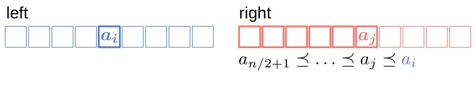
6.1. The Merge Step

We count cross-inversions in the merge step. Since $left$ and $right$ are sorted after the recursion, if $a_i \not\preceq a_j$ and $a_i \in left \land a_j \in right$ , it holds that $a_i$ is in inversions with $b_j$ and its predecessors in $right$ :

Since the indices in $right$ start with $n/2$ , we subtract that offset from $j$ and add the difference to the count.

6.2. Complexity

The algorithm’s time complexity is $O(n \log n)$ like that of Merge Sort, which beats the straightforward $O(n^2)$ method.

It’s usually slower than the sampling approach but returns the same value over multiple runs. Therefore, this implementation might be the middle ground between the sampling’s performance and the quadratic algorithm’s exactness.

Unlike the previous two approaches, this one solves an additional problem (sorting an array) to handle the original one. So, it does more work than necessary.

7. Alternative Measures

A computationally lightweight approach would be to consider only the inversions with successive elements:

$a_i \not\preceq a_{i+1}$

There are at most $n-1$ such inversions, and we need only one traversal over the array to count them, checking the successive pairs. So, the time complexity will be $O(n)$ , but this measure might not give us a clear picture of an array’s sortedness. The reason is that out-of-order elements at the beginning of $a$ can participate in more inversions than those near the end, but this metric treats all pairs equally.

Another approach is to calculate the rank distance. Let $a'$ be the sorted permutation of $a$ , and let $r_i$ be the rank of $a_i$ in the $a$ , which we can find by looking it up in $a'$ (we use averages for non-unique elements). Then, the rank distance can be computed as the Euclidean distance between the original indices and ranks:

$\sqrt\{\sum_{i=1}^{n}(i-r_i)^2\}$

or the average absolute difference:

$\frac{1}{n}\sum_{i=1}^{n}|i - r_i|$

A shortcoming of this approach is that we need to sort $a$ to find the ranks.

8. Conclusion

In this article, we showed how to define and compute the sortedness of an array. A natural measure of it is the count of inversions. There are stochastic and deterministic ways to calculate it.

We should use the sampling approaches if we’re more concerned about performance.

Full Archive

About Baeldung

Core Concepts

Operating Systems

Artificial Intelligence

Graph Theory

Latex