

Learn through the super-clean Baeldung Pro experience:
>> Membership and Baeldung Pro.
No ads, dark-mode and 6 months free of IntelliJ Idea Ultimate to start with.
Last updated: March 18, 2024
Learn through the super-clean Baeldung Pro experience:
>> Membership and Baeldung Pro.
No ads, dark-mode and 6 months free of IntelliJ Idea Ultimate to start with.
In this tutorial, we’ll discuss finding the intersection of linked lists. In the beginning, we’ll discuss different approaches to finding the intersection of two lists.
After that, we’ll show how to generalize these approaches to find the intersection of multiple lists.
Finally, we’ll end with a comparison that shows the main differences between the discussed approaches.
We need to define the intersection of multiple lists. Let’s take the following example:
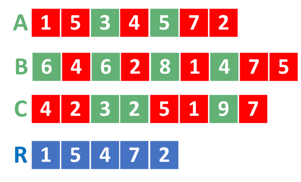
In the example, we have three lists  ,
,  , and
, and  . Also, we have
  , which represents the intersection of the previous three ones.
To calculate the intersection of multiple lists, we need to determine the mutual elements between them. In the example above, the mutual elements are marked with a red color.
One thing to note here is the case of a value being repeated more than once. In this case, the resulting must contain it with the minimum number of its repetitions. For example, if a value is repeated two times in , three times in , and two times in , then will contain it two times.
Thus, the problem reduces to finding the intersection of some given lists. For simplicity, we’ll discuss many approaches to solving the problem in the case of two lists first.
After that, we’ll see how to generalize all the discussed approaches so that they can handle multiple lists.
In the naive approach, we’ll iterate over all the elements of the first list. For each element, we check whether it exists inside the second one.
Consider the implementation of the naive approach:
algorithm naiveIntersection(A, B):
    // INPUT
    //   A = The first list
    //   B = The second list
    // OUTPUT
    //   Returns the intersection of lists A and B

    R <- an empty list
    iter <- A.head

    while iter != null:
        if B.contains(iter.value):
            R.add(iter.value)
            B.erase(iter.value)
        iter <- iter.next

    return R
First of all, we define as an empty list that will hold the answer to the problem. Also, we set an iterator  that points to the beginning of .
After that, we iterate over all the elements of . For each element, we check whether contains an element of the same value. If so, we add the element to the resulting .
Also, we delete the element from . Note that the  function should only delete the first appearance of the element from
  . The reason is that if the element was repeated more than once in both and , we need to add twice to .
Once we’re done checking the element, we move the iterator forward to the next element.
Finally, we return the resulting .
The complexity of the naive approach is  , where
  is the number of elements in and
  is the number of elements in .
The reason is that is not sorted. Hence, we need to perform a linear search to check the existence of each element.
In the naive approach, we performed a linear search operation inside to find whether an element exists inside it or not. Let’s think about how to improve this search.
We can add the elements inside to a TreeSet and then perform a quick search inside it. However, this would cause repeated elements to be added only once. Therefore, we won’t be able to handle the case of repeated elements.
Another way would be to add all the elements inside to a TreeMap or a HashMap. In this tutorial, we’ll go with the TreeMap.
The idea is to calculate the number of repetitions of each element inside . For example, if the value five is repeated three times inside , then we’d have ![map[5] = 3](/wp-content/ql-cache/quicklatex.com-2a5a0bc1a3229ac908775bab292a9702_l3.svg "Rendered by QuickLaTeX.com") .
.
Now, we can simply check the existence of some value inside by checking its repetition. If the repetition is larger than zero, then the value exists, and we can add it to the answer.
Also, removing the first appearance of the value from becomes easier as well. To erase an element from  , we decrease its repetitions by one.
Let’s take a look at the implementation of the faster approach:
algorithm fasterIntersection(A, B):
    // INPUT
    //   A = The first list
    //   B = The second list
    // OUTPUT
    //   Returns the intersection of lists A and B

    map <- an empty map with default value 0
    iter <- B.head

    while iter != null:
        map[iter.value] <- map[iter.value] + 1
        iter <- iter.next

    R <- empty list
    iter <- A.head
    while iter != null:
        if map[iter.value] > 0:
            R.add(iter.value)
            map[iter.value] <- map[iter.value] - 1
        iter <- iter.next

    return R
Similarly to the naive approach, we initialize the empty list that will hold the resulting answer to the problem. Also, we initialize the map with zero. The reason is that if we were to look up the repetition of some value, and it wasn’t added yet, the map should return the default value, which is zero.
Next, we iterate over all the elements inside . For each element, we increase the repetition of its value by one inside the map and move to the next one.
After that, we iterate over all the elements inside . For each element, we check whether the repetition of its value inside  is larger than zero. If so, we add it to the resulting and decrease its repetition by one. Also, we move the iterator one step forward to reach the next element.
Finally, we return the resulting .
The complexity of this approach is  , where is the number of elements inside the first list, and is the number of elements inside the second one.
Note that it’s always optimal to add the larger list to the map, and iterate over the smaller one. The reason is that  .
.
Let’s describe some special cases to the problem. Since the faster approach has a better complexity, we’ll discuss the improvements over it rather than the naive approach.
Suppose the elements inside the lists were small integer values. In this case, we don’t need to use a TreeMap. Instead, we can just use an array of size  , where is the maximum value inside and .
Therefore, the variable  inside algorithm 2 should be an array, rather than being a TreeMap. For initialization, we must initialize all the elements inside this array with zeroes. After that, we iterate over the elements of and increase the repetition of its values by one.
The implementation stays the same, except for the concept that is now an array.
Note that if one of the lists contains smaller values than the other, it’s optimal to calculate repetitions for this array. The reason is that the value of will be smaller.
Also, we need to update the algorithm a little. When iterating over the elements of  , if one of the elements is larger than
  , we immediately continue without checking its repetition. The reason is that its repetition will surely be zero, and we don’t want to go out of the range of the array .
The complexity of this approach is  , where is the size of the first list, is the size of the second one, and is the maximum value in one of them, whichever has the lowest one.
The second special case is when we have both lists sorted. In this case, we can come up with a completely new approach.
We’ll iterate over both lists at the same time. In each step, we’ll move the iterator of the one whose value is smaller. If both iterators reach the same value, we add it to the result and move both iterators.
Take a look at the implementation of this approach:
algorithm sortedListsIntersection(A, B):
    // INPUT
    //   A = The first list
    //   B = The second list
    // OUTPUT
    //   Returns the intersection of lists A and B

    R <- empty list
    aIter <- A.head
    bIter <- B.head

    while aIter != null and bIter != null:
        if aIter.value < bIter.value:
            aIter <- aIter.next
        else if bIter.value < aIter.value:
            bIter <- bIter.next
        else:
            R.add(aIter.value)
            aIter <- aIter.next
            bIter <- bIter.next

    return R
Same as before, we initialize the empty list to contain the resulting answer. However, in this approach, we obtain two iterators  and
and  to iterate over both and .
In each step, we move forward the iterator that points to a smaller value. Nevertheless, if both iterators point to two elements whose values are equal, then we add this value to the result and move both iterators.
The idea behind this approach is that, if both iterators are pointing to different values, then we must move one of them. However, since both lists are sorted, the smaller value can’t be found anymore inside the other list. The reason is that the iterator of the other one already points to a larger value.
Therefore, it’s always optimal to move the one that points to a smaller value.
The complexity of this approach is  , where is the number of elements inside the first list and is the number of elements inside the second one.
In case we’re given more than two lists and need to calculate the intersection of all of them, we can update any of the previously described approaches.
In the beginning, we can calculate the intersection of the first two lists using any of the described approaches. Next, we can calculate the intersection of the result, with the third one, and so on.
This operation continues until we reach the final result.
The complexity of using this approach is related to the complexity of calculating the intersection of every two lists. However, we should add up the complexity of each step individually.
For example, if we had three lists, and we were able to use the sorted lists approach, the complexity will be  , where is the size of the first one, is the size of the second, and
  is the size of the third.
Let’s take a look at a comparison between all the previously discussed approaches:
| Naive Approach | Faster Approach | Small Integers Approach | Sorted Lists Approach | |
|---|---|---|---|---|
| Time Complexity |  |
 |
 |
 |
| Memory Complexity |  |
 |
 |
|
| Use Cases | General approach | General approach | Only when the values in one of the lists are relatively small | Only for sorted lists |
Note that the memory complexity describes the extra memory allocated by the algorithm. Thus, it doesn’t describe the memory allocated by both lists.
As we can see, in the general case, using the faster approach is always recommended as it has low complexity, and doesn’t consume larger memory than the one already consumed by both lists.
However, both the small integers approach and the sorted lists approach are useful in their respective special cases.
When the values of at least one of the lists are small, then we should consider using the small integers approach. However, we must pay attention that, in this case, we’re allocating memory of  . This memory must be relatively small to be able to use this approach.
On the other hand, if they’re sorted, then we should use the sorted lists approach as it provides the lowest complexity, and doesn’t consume extra memory.
In this tutorial, we discussed the problem of finding the intersection of linked lists. Firstly, we described the naive approach and improved it to obtain a better one.
Secondly, we presented some special cases and showed the updates needed to implements each of them.
Thirdly, we explained how to update all the approaches to obtain the intersection of multiple lists.
Finally, we summarized with a comparison table that listed the main differences between all the discussed approaches.