

Yes, we're now running our only Summer Sale. All Courses are 30% off until 20th July, 2026:
Learn through the super-clean Baeldung Pro experience:
>> Membership and Baeldung Pro.
No ads, dark-mode and 6 months free of IntelliJ Idea Ultimate to start with.
1. Introduction
Flowcharts are an excellent resource for systematically illustrating processes and algorithms. With flowcharts, we can define, for instance, conditional decisions and loopings in a visual and simple way.
LaTeX, in summary, is a system that uses tags and marks to format a document. Several packages are available for LaTeX, including different drawing packages. These drawing packages enable the users to create several graphical resources from scratch.
Among these packages, there exists the one called TikZ. TikZ is a vector drawing package for general use. In particular, TikZ provides multiple tools for drawing flowcharts.
In this tutorial, we will explore how to draw flowcharts using LaTeX/TikZ. At first, we’ll study the organization of a LaTeX/TikZ picture environment. So, we’ll see a set of TikZ elements usable for drawing flowcharts. Finally, we’ll have some examples of complete TikZ flowcharts.
2. The LaTeX/TikZ Picture Environment
Drawing with LaTeX/TikZ requires importing specific packages and organizing the environment with particular tags. In this way, this section presents how to prepare a LaTeX document to draw flowcharts with TikZ.
In our examples, we will use the following code as the base document to draw flowcharts:
(1) \documentclass{standalone}
(2) \usepackage{tikz}
(3) \usetikzlibrary{shapes, arrows}
(4) \begin{document}
(5) \begin{tikzpicture}
(6) ...
(7) \end{tikzpicture}
(8) \end{document}
Our base document uses the standalone class (line 1). Thus, the LaTeX compiler will create a PDF particularly for the TikZ image defined in the document. However, we can employ TikZ with other document classes with no problems, such as article and a4paper.
In the following line (2), we import the TikZ package to the LaTeX document. This importing line enables us to use the TikZ resources. Line 3, in turn, specifies that we’ll use the shapes and arrows library from TikZ.
Note that it is common to use TikZ to draw charts and graphs besides flowcharts.
Next, we can open the environments of our example document. Line 4 defines the beginning of the LaTeX document itself. Line 5, in turn, indicates the begging of a TikZ picture environment.
After opening our environments, we can define the TikZ image. In our example, line 6 represents the image definition. But, it is relevant to notice that this definition can have multiple lines.
Finally, lines 7 and 8 show the end of the TikZ picture environment (7) and the LaTeX document (8).
We highlight that, by default, the LaTeX compiler generates PDF documents. However, in the case of standalone images, it is possible to convert them to other file formats, such as PNG and JPG.
2.1. LaTeX/TikZ Coordinate System
Creating flowcharts with TikZ consists of including graphical elements into an image. Thus, we must consider an image origin point as a referential to properly allocate these elements.
For drawing our flowcharts, we’ll consider the 2D coordinate system (X, Y) of the TikZ package. In the following image, we can see a simple cartesian plane system of TikZ:
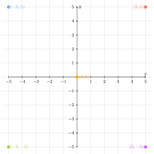
The origin of the cartesian plane of TikZ is at the middle of the image (yellow point). Taking the origin point as the referential, the coordinate system to locate graphical elements in the image behaves as follows:
- Positive X and Y: the middle point of the graphical element will be located at the upper-right section of the cartesian plane (for example, red circle)
- Negative X and Y: the middle point of the graphical element will be located at the lower-left section of the cartesian plane (for example, green circle)
- Negative X and positive Y: the middle point of the graphical element will be located at the upper-left section of the cartesian plane (for example, blue circle)
- Positive X and negative Y: the middle point of the graphical element will be located at the lower-right section of the cartesian plane (for example, purple circle)
3. Flowchart Elements in TikZ
There are several elements for drawing flowcharts. These elements are, at most, simple geometrical figures. In this section, we’ll explore some of these flowchart elements in the context of LaTeX and TikZ.
It is relevant to highlight that, in the following subsections, we will show the definition command to create flowchart elements using TikZ. Therefore, we should include the definition commands before the begin document command in the LaTeX file (\begin{document}).
3.1. Terminator
The terminator element indicates the beginning or end of a process. To define a terminator in TikZ, we can use the following definition command:
\tikzstyle{terminator} = [rectangle, draw, text centered, rounded corners, minimum height=2em]Next, we can see the terminator element image:

Finally, we can include this element as a node in a TikZ picture environment as follows:
\node at (X,Y) [terminator] (t-id) {Terminator};3.2. Process
The process element represents a processing function in the flowchart. So, the TikZ definition line for the process element is presented next:
\tikzstyle{process} = [rectangle, draw, text centered, minimum height=2em]The following image depicts the process element:

We can reproduce the image in a TikZ picture environment with the subsequent command:
\node [process] at (0,0) (p-id) {Process};3.3. Decision
The decision element represents two or more branches on the flowchart. Thus, it defines different paths taken according to particular conditions. We can define the decision element with the line in next:
\tikzstyle{decision} = [diamond, draw, text centered, minimum height=2em]The image shown next depicts the decision element:

With the previous definitions done, we can insert the decision element in the flowchart using the following command:
\node [decision] at (X,Y) (d-id) {Decision};3.4. Data
The data element indicates an operation of input or output in the flowchart. So, this element means that data is being introduced to or provided by the system. A viable manner to define this element is presented next:
\tikzstyle{data}=[trapezium, draw, text centered, trapezium left angle=60, trapezium right angle=120, minimum height=2em]The image below demonstrates the data input/output element:

The following line inserts a data element into a flowchart:
\node [data] at (X,Y) (dio-id) {Data\\In/Out};3.5. Connector
The connector element consists of the relationship between elements. Following a set of connectors of the flowchart, in turn, create paths. We can see the definition of the connector element next:
\tikzstyle{connector} = [draw, -latex']The following image presents the connector element shape:
We can use the subsequent line to produce a connector between two elements (e1-id as the origin and e2-id as the destination):
\path [connector] (e1-id) -- (e2-id);We highlight that the double hyphen between the elements indicates a straight line connecting them. To create curved lines in the flow chart, we can replace one hyphen with a pipe: |- or -|.
4. Simple Flowcharts Examples
In this section, we’ll see different ways to create flowcharts using the elements shown in the previous section. At first, we’ll understand how to build a flowchart explicitly defining the coordinates of the elements. So, we’ll build the same flowchart through relative positions instead of explicit coordinates.
4.1. Creating Flowcharts With Explicit Coordinates
Using the coordinates, we can place the elements in any location of the TikZ cartesian plane with no restrictions. Thus, employing explicit coordinates makes the process of creating flowcharts very generic and customizable.
The following LaTeX/TikZ code shows the TikZ picture environment to create a simple flowchart using explicit coordinates:
\begin{tikzpicture}
\node [terminator, fill=blue!20] at (0,0) (start) {\textbf{Start}};
\node [data, fill=blue!20] at (0,-2) (data) {Provide data};
\node [decision, fill=blue!20] at (0,-5) (decision) {Valid data?};
\node [process, fill=red!20] at (3.5,-5) (error) {Error};
\node [process, fill=green!20] at (0,-8) (success) {Success};
\node [terminator, fill=blue!20] at (0,-10) (end) {\textbf{End}};
\node[draw=none] at (1.85, -4.75) (no) {No};
\node[draw=none] at (0.35, -6.75) (yes) {Yes};
\path [connector] (start) -- (data);
\path [connector] (data) -- (decision);
\path [connector] (decision) -- (error);
\path [connector] (decision) -- (success);
\path [connector] (error) |- (end);
\path [connector] (success) -- (end);
\end{tikzpicture}
The image below depicts the flowchart generated by the previously presented code:
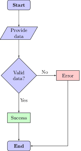
The flowchart contains a total of 12 elements: two terminators (start and end), one data element (data), one decision element (decision), two processes (error and success), and six connectors.
The coordinates of the elements were explicitly defined (at (X, Y)). The exception, however, is the connectors. Connectors don’t require coordinates definition, only the identifiers of the elements they connect.
We also employed the node modifier fill to set colors for the elements. Furthermore, we used extra nodes for labeling specific connectors (no and yes).
4.2. Creating Flowcharts With Relative Positioning
Despite decreasing the customization possibilities compared to explicitly defining coordinates, the relative positioning of elements in a flowchart can bring several advantages.
Among these advantages, we can cite, for example, the intuitiveness of building flowcharts and the standardization of the distance between elements in the flowchart.
The following LaTeX/TikZ code shows the TikZ picture environment to create a simple flowchart using relative positioning:
\begin{tikzpicture}[node distance = 3cm]
\node [terminator, fill=blue!20] (start) {\textbf{Start}};
\node [data, fill=blue!20, below of=start] (data) {Provide data};
\node [decision, fill=blue!20, below of=data] (decision) {Valid data?};
\node [process, fill=red!20, right of=decision] (error) {Error};
\node [process, fill=green!20, below of=decision] (success) {Success};
\node [terminator, fill=blue!20, below of=success] (end) {\textbf{End}};
\node[draw=none] at (1.60, -5.75) (no) {No};
\node[draw=none] at (0.35, -7.80) (yes) {Yes};
\path [connector] (start) -- (data);
\path [connector] (data) -- (decision);
\path [connector] (decision) -- (error);
\path [connector] (decision) -- (success);
\path [connector] (error) |- (end);
\path [connector] (success) -- (end);
\end{tikzpicture}
The image generated using the previously presented code is presented next:
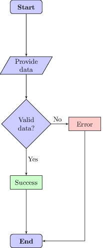
It is relevant to note that the definition of coordinates got replaced with node positioning modifiers (below of, above of, right of, left of). So, we need to provide a referential allocate an element.
The referential, in our case, is any other previously allocated element, and the global referential is the first allocated element (the terminator start).
Furthermore, we employ the TikZ picture environment modifier of node distance to determine the standard distance between neighbor node centers.
Finally, we defined the coordinates of the labeling nodes (no and yes) once they demand a specific positioning on the image.
5. Conclusion
In this tutorial, we learned about drawing flowcharts with LaTeX/TikZ. First, we took a look at how the LaTeX/TikZ environment works. Thus, we mainly studied some elements used to build flowcharts, observing how to create them with LaTeX/TikZ. Finally, we attempted how to build complete flowcharts with these elements.
We can conclude that LaTeX/TikZ is a very versatile tool to create flowcharts. Specifically, the TikZ package library enables the user to create several forms natively, and its libraries provide several of these forms already defined.