Interpolation Search | Baeldung on Computer Science

1. Introduction

In this tutorial, we’ll delve into the workings of the Interpolation Search algorithm, exploring its principles, advantages, and limitations.

2. The Need for Efficient Searching Algorithms

In the vast landscape of computer science and data analysis, quickly locating desired information is vital. Searching algorithms are at the core of various applications, from simple data structures to databases.

A fundamental requirement for searching algorithms is efficiency, especially when dealing with massive datasets where the search time can become a bottleneck. The classical searching methods, such as linear and binary searches, have served well, but they aren’t optimal in all cases:

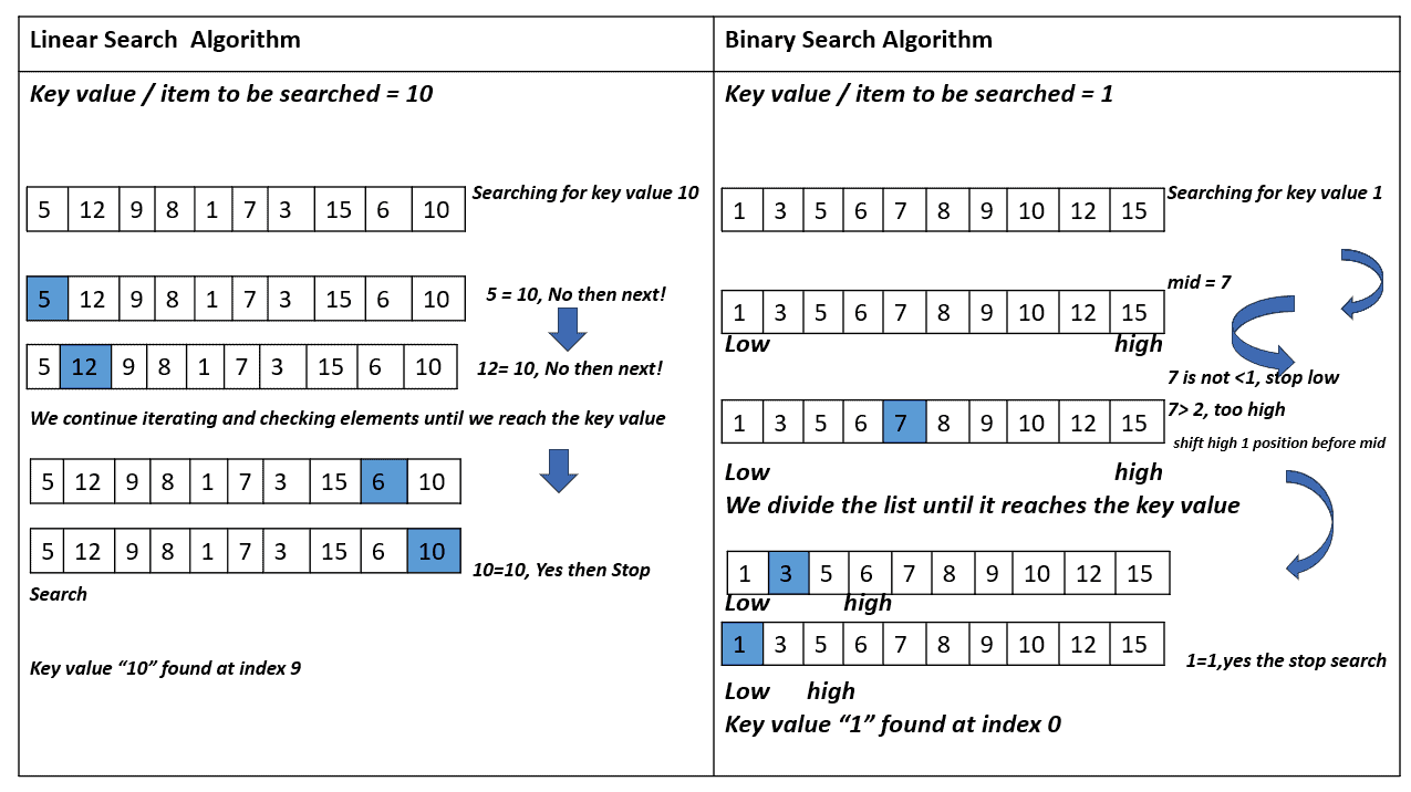
In the case of linear search, we need to iterate through the entire list, checking each element until we reach the target at the end of the array. This is the worst-case scenario for linear search.

Similarly, binary search will continually divide the array in half until it reaches the position of the target. In our example, that’s the first element. However, the target’s actual position could be found faster if binary search adapted to the values in the array.

The Interpolation Search algorithm has been designed to overcome the limitations of traditional search methods and enhance search efficiency for large datasets. It uses mathematical interpolation to estimate the position of the target element, potentially leading to faster search times.

3. Overview of the Interpolation Search Algorithm

This algorithm combines Binary Search with linear interpolation, making it suitable for sorted arrays and effectively handling non-uniformly distributed values.

It determines the target element’s position based on its value and the extreme values within the currently searched section of the array. Subsequently, this estimated position undergoes further refinement in successive steps until the target is found or considered absent. Compared to Linear Search, Interpolation Search covers more significant portions of the input array with each step.

3.1. Pseudocode

Here’s the pseudocode:

The algorithm repeatedly estimates the position of the target element based on its value and the values at the extremes of the search portion of the array. It stops if it finds the element or infers it isn’t in the array.

3.2. The Mathematics Behind Interpolation Search

The efficiency of the Interpolation Search algorithm lies in its mathematical formula, which estimates the position of the target element. Given a sorted sub-array with start and end indices $low$ and $high$ , and a target value $target$ , the estimated position $pos$ of $target$ is:

$pos = low + \left\lceil \frac{(target - arr[low]) \cdot (high - low)}{arr[high] - arr[low]}) \right\rceil$

Here, $arr$ is our sorted array. We round the index to the nearest lower integer since the fraction might be float, and indices are integers.

3.3. Example

Let’s say we have a sorted array of integers: $[10, 20, 30, 40, 50, 60, 70, 80, 90, 100]$ . Our target element is 60, and we want to find its index using Interpolation Search.

Initially, we set the search range to $low = 0$ and $high = length(arr) - 1 = 9$

Then, we calculate the estimated position using linear interpolation:

$low + ((target - arr[low]) (high - low)/ (arr[high] - arr[low])) = 0 + ((60 - 10) (9 - 0)/ (100 - 10)) = 5$

Since $arr[5]=60$ , we have found the element and return 5 as its index.

4. Complexity Analysis

Understanding the complexity of the Interpolation Search algorithm is crucial to evaluating its efficiency and applicability in various scenarios.

In the best case, the array is uniformly distributed, and the target element is found early. So, Interpolation Search approaches the time complexity of $O(1)$ . This is because the estimated position often leads directly to the target.

Conversely, in the worst case, the Interpolation Search may behave as Linear Search, mainly when dealing with non-uniformly distributed data. In some non-uniform cases, the time complexity could be $O(n)$ , where $n$ is the size of the input array.

Turning to the average case, the time complexity of Interpolation Search is approximately $O(\log \log n)$ for uniformly distributed data, which is an improvement over $O(\log n)$ of Binary Search.

4.2. Space Complexity

The space complexity is low. It’s $O(n)$ since we need to store the input array and have a constant number of auxiliary variables (such as $low, high, pos$ ).

5. Advantages of Interpolation Search

The Interpolation Search algorithm offers several advantages over traditional searching methods,

5.1. Speed and Efficiency

Interpolation Search exhibits excellent performance for uniformly distributed arrays.

Each step covers larger portions of the array, leading to faster convergence toward the target.

5.2. Efficient for Large Arrays

The algorithm’s efficiency becomes more pronounced as the array size increases.

Linear search may become impractical for large datasets, but Interpolation Search can still provide reasonable search times.

5.3. Early Exit

If the target element isn’t in the array, Interpolation Search may identify this early and terminate the search sooner.

5.4. Adaptability to Non-Uniform Arrays

This search technique efficiently estimates the target’s location by considering array distribution.

It computes proportional intervals, enabling precise targeting in skewed datasets. It’s responsive to irregular data distributions. This adaptability enhances search efficiency across varying array structures, making interpolation search a versatile choice for non-uniform datasets.

6. Limitations and Constraints

Despite its efficiency, Interpolation Search has some limitations we need to consider.

6.1. Non-Uniformly Distributed Data

The array values should be uniformly distributed for the algorithm to perform optimally.

It still works in non-uniform cases, but its efficiency may decline depending on the distribution. That’s because estimating the target’s position can become less precise due to uneven value distribution, potentially requiring more interpolation steps. Its complexity approaches $O(n)$ for some non-uniform distributions.

6.2. Sortedness Prerequisite

The Interpolation Search algorithm requires a sorted array to operate correctly.

If the array isn’t sorted, it must be sorted first, adding an initial overhead.

7. Conclusion

In this article, we explored the interpolation search algorithm. The Interpolation Search algorithm offers a compelling alternative to traditional searching techniques such as Binary Search and Linear Search.

By estimating the probable position of the target element within the sorted array, Interpolation Search offers a more efficient approach for large datasets. Despite its limitations, the algorithm has found significant applications in various real-world scenarios, especially when speed and precision are crucial.

While it excels in uniformly distributed datasets due to its accurate position estimation, its performance can be less reliable in non-uniform cases, contingent on the data distribution.

Full Archive

About Baeldung

Core Concepts

Operating Systems

Artificial Intelligence

Graph Theory

Latex