Differences Between Homography and Affine Transformation

1. Overview

In computer vision and image processing, affine transformation and homography are essential techniques used to align images and correct geometric distortions.
In this tutorial, we’ll recall the mathematical definitions of affine transformation and homography. Then we’ll explain the difference between them by providing illustrative examples.

2. Affine Transformation

An affine transformation is represented by a function composition of a linear transformation with a translation.
The affine transformation of a given vector $mathbf{x} in mathbb{R}^n$ is defined as:

$mathbf{x}' =mathbf{A} mathbf{x} +mathbf{b}$

where $mathbf{x}' in mathbb{R}^n$ is the transformed vector, $mathbf{A}$ is a square and invertible matrix of size $n times n$ and $mathbf{b}$ is a vector of size $n$ .
In geometry, the affine transformation is a mapping that preserves straight lines, parallelism, and the ratios of distances. This means that:

points on the same line initially, lie on a line after the transformation
parallel lines before the transformation remain parallel after the transformation
the ratio of any pair of segments remains the same after the transformation. Hence, the midpoint of a segment remains the midpoint.

On the other hand, affine transformations do not necessarily preserve lengths and angles.
The following figure shows an example of an affine transformation applied to a checkered image:

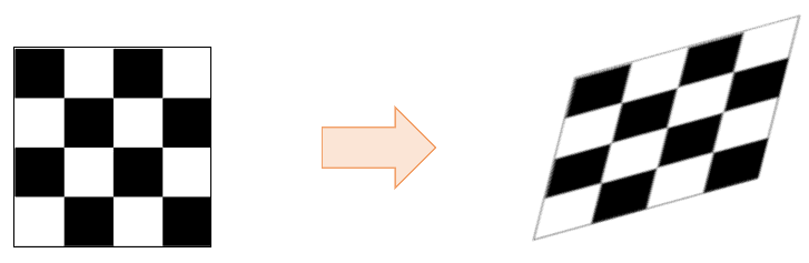
In the 2D case, the affine transformation is given by the equations:

$begin{cases} x' = a_{11} x +a_{12}y + b_1 \ y' = a_{21}x + a_{22}y + b_2 end{cases}$

that can be expressed in a single product matrix-vector using the homogeneous coordinates:

$left[begin{array}{l} x' \ y' \ 1 end{array}right] = left[begin{array}{lll} a_{11} & a_{12} & b_{1} \ a_{21} & a_{22} & b_{2} \ 0 & 0 & 1 end{array}right] left[begin{array}{l} x \ y \ 1 end{array}right]$

The matrix elements of the affine transform have the following meanings:

$a_{11}$ : scaling in the $x$ -direction
$a_{12}$ : shearing in the $x$ -direction
$b_{1}$ : translation in the $x$ -direction
$a_{21}$ : shearing in the $y$ -direction.
$a_{22}$ : scaling in the $y$ -direction.
$b_{2}$ : translation in the $y$ -direction.

Translation, scaling, rotation, and shearing are particular types of affine transformations. In fact, a translation is represented by a matrix of the form:

$T = left[begin{array}{lll} 0 & 0 & t_{x} \ 0 & 0 & t_{y} \ 0 & 0 & 1 end{array}right]$

while the scaling matrix is:

$C = left[begin{array}{lll} C_x & 0 & 0 \ 0 & C_y & 0 \ 0 & 0 & 1 end{array}right]$

and the shearing matrix is:

$S = left[begin{array}{lll} 0 & s_x & 0 \ s_y & 0 & 0 \ 0 & 0 & 1 end{array}right]$

3. Homography

The homography, also known as perspective transform, is a geometric transformation that relates two different planes:

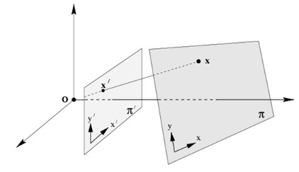
Looking at the figure above, each point $mathbf{x} = (x, y)$ of the plane $mathbf{pi}$ is related to a point $mathbf{x'} = (x', y')$ in the plane $mathbf{pi'}$ using the following equation operating on the homogeneous coordinates:

$left[begin{array}{c} s x^{prime} \ s y^{prime} \ s end{array}right]=mathbf{H}left[begin{array}{l} x \ y \ 1 end{array}right]$

where $s$ is a scale factor and $mathbf{H}$ is a $3 times 3$ matrix called the homography matrix:

$left[begin{array}{lll} h_{11} & h_{12} & h_{13} \ h_{21} & h_{22} & h_{23} \ h_{31} & h_{32} & h_{33} end{array}right] .$

Two homography matrices are equivalent if they differ only by a scale factor. Hence, the matrix $mathbf{H}$ is generally normalized with $h_{33}=1$ .
The inhomogeneous coordinates of the transformed point $mathbf{x}'$ are computed as follows:

$x^{prime}=frac{h_{00} x+h_{01} y+h_{02}}{h_{20} x+h_{21} y+h_{22}} quad text { and } quad y^{prime}=frac{h_{10} x+h_{11} y+h_{12}}{h_{20} x+h_{21} y+h_{22}} text {. }$

Homography is a mapping that preserves straight lines, i.e., points that are on the same line initially lie on a line after the transformation.
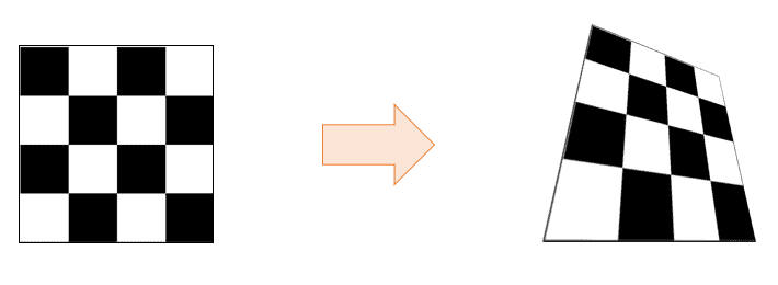
The following figure shows an example of homography applied to a checkered image:

4. Difference

While both affine transformation and homography are types of geometric transformations that can be used to map one image onto another, there are some key differences between them:
An affine transformation preserves straight and parallel lines, while homography preserves only straight lines. This means that points that are collinear before an affine transformation remain collinear after the transformation, but this is not necessarily the case for homographies.
Another difference is the number of degrees of freedom. An affine transformation has 6 degrees of freedom, as it can be represented by a $2 times 3$ matrix with 6 coefficients. A homography has 8 degrees of freedom, as it can be represented by a $3 times 3$ matrix with eight free parameters.
The third difference is the type of distortion they can correct. Affine transformations can correct for translations, rotations, shears, and scales, but they cannot be correct for perspective distortion. Homographies, on the other hand, can correct for perspective distortion, as well as translations, rotations, shears, and scales.

5. Applications

Here are some applications of affine transformation and homography in computer vision and image processing:

Image alignment and registration: affine transformation and homography can be used to align and register images by computing the transformation matrix using a set of corresponding points in the source and target images. This is useful in tasks such as image stitching, panorama creation, and object recognition
Perspective correction: homography can be used to correct perspective distortion in images. This is useful in tasks such as aerial imaging, street view mapping, and augmented reality
Object tracking: affine transformation and homography can be used to track objects in images by estimating the transformation matrix between consecutive frames and using it to predict the location of the object in the next frame
Medical imaging: affine transformations are used to align and register medical images, such as CT scans and MRIs, to improve the accuracy of diagnosis and treatment planning
Remote sensing: affine transformation and homography can be used to align and register satellite images by computing the transformation matrix using a set of corresponding points in the source and target images
Robotics: affine transformation and homography can be used in robotics to align and register images from different sensors, such as cameras and lidars, to improve the accuracy of localization and mapping

6. Conclusion

In this article, we reviewed affine transformation and homography, two essential techniques used to align and correct geometric distortion in images. We discussed their differences and provided their main applications in image processing and computer vision.

Learn Java Collections

Learn Spring

Learn Maven

View All Courses

Core Concepts

Operating Systems

Neural Networks

Graph Theory

Latex

Full Archive

About Baeldung