Gravity/Bead Sort

1. Introduction

In this tutorial, we’ll learn about the gravity sort algorithm, also known as bead sort.

We use many sorting algorithms to arrange data in a particular order in our applications. Gravity sort is a natural sorting algorithm because natural phenomena – in this case, the force of gravity – inspired its design and development.

Natural sorting algorithms show us that we can develop ideas by observing nature. We can also learn a lot from the challenges of adapting such algorithms to software.

2. Gravity Sort

Gravity sort was developed in 2002 by Joshua J. Arulanandham, Cristian S. Calude, and Michael J. Dinneen. Natural events inspired the researchers to develop an algorithm for sorting positive integers. As they observed in their research paper, the force of gravity creates a “natural comparison” between positive integers that results in a sorted list. In other words, by simulating gravity on a list of positive integers, we can sort them.

To understand this, let’s represent positive integers as sets of beads suspended on abacus rods. For example, as we see in the image on the left, we’d represent the number three by hovering three beads in the air across three rods and the number two as two beads across two rods. When gravity acts upon the beads, any bead without another bead under it will fall. We can see the result of this below in the image on the right:

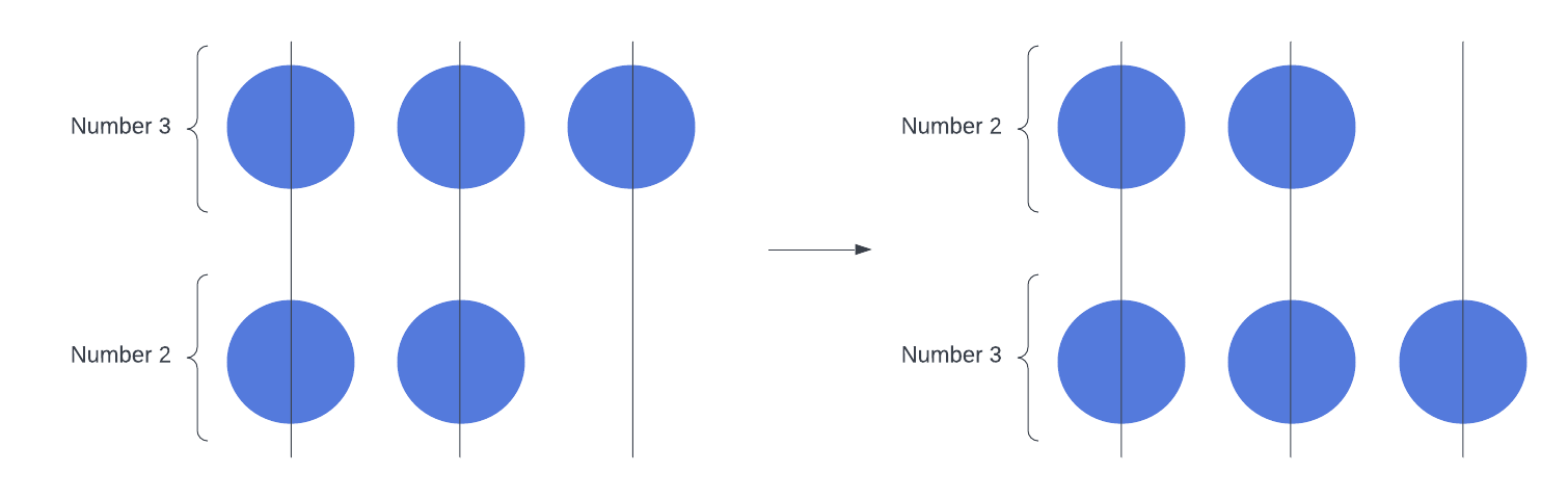
After the third bead of the number three has fallen, it’s now part of the bottom number. The resulting state of the abacus represents the same set of positive integers, but gravity has sorted those integers in ascending order.

Let’s look at a more complex example:

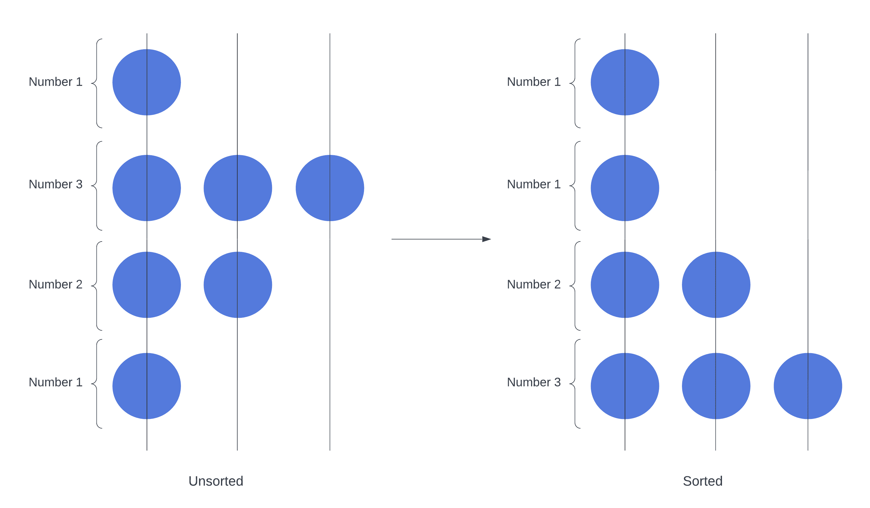
The image to the left represents the unsorted list of numbers. From top to bottom, the numbers are . On the right, we can see the final state after the beads have fallen down the rods: . Gravity has sorted our numbers.

Let’s look at how we can model this phenomenon in software.

3. Algorithm

To simulate an abacus, we use a 2D matrix to represent a system of vertical rods and horizontal levels. The state of a given cell is either occupied or empty based on whether it contains a bead. An on-bit indicates a bead is in the cell, and an off-bit is an empty cell.

Given a list of positive integers, , and is the biggest number in , the abacus will have at least rods and levels in the matrix.

Let’s walk through a specific example using the list . First, we process to create the initial state of the matrix: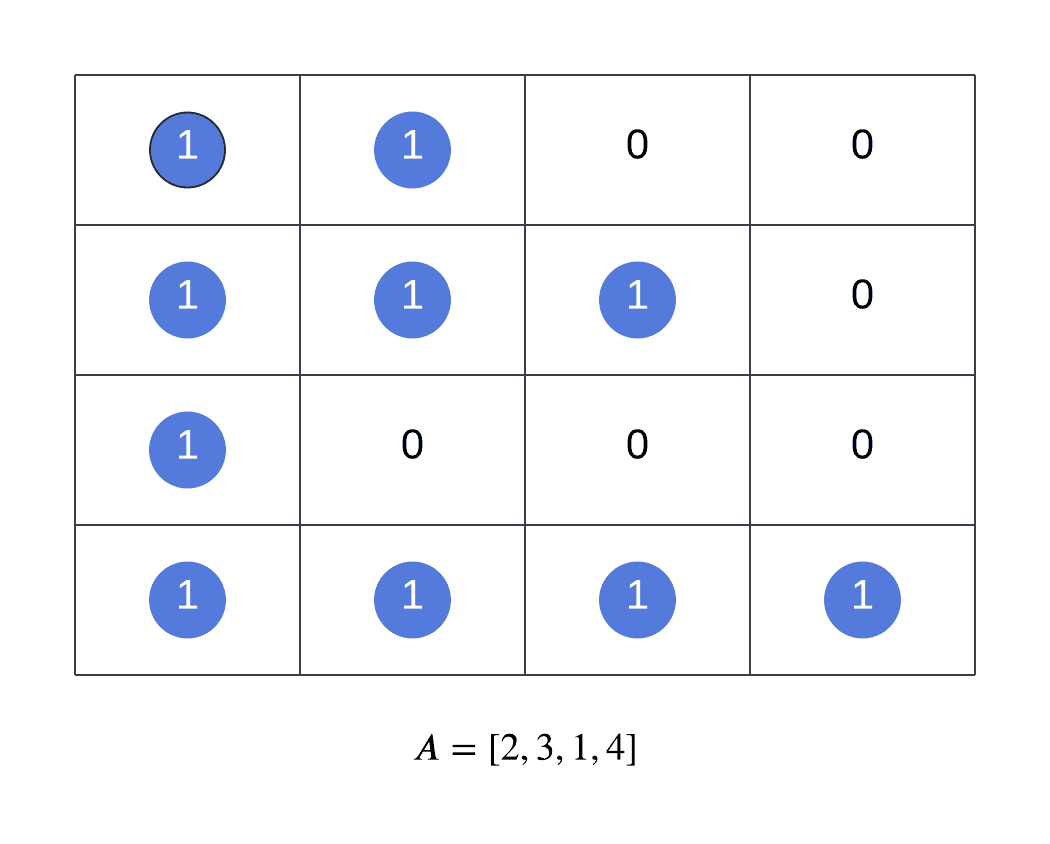

Starting at , where is the current level at each passing of the gravity sort algorithm, the matrix evolves as follows: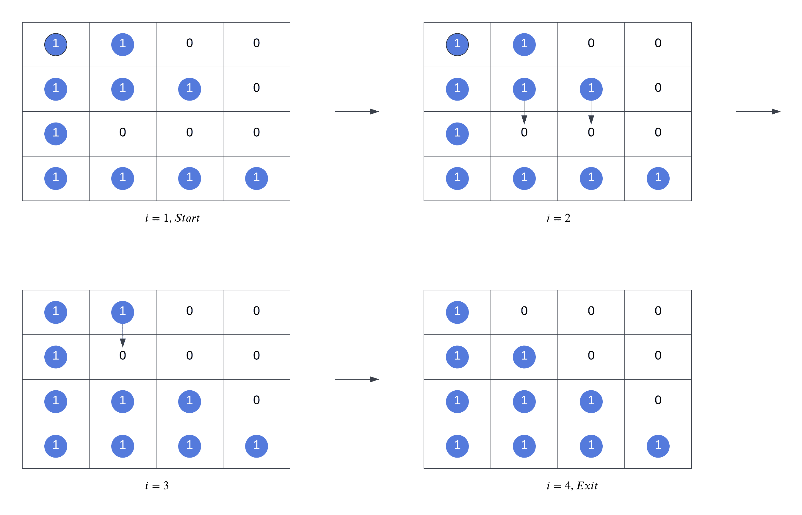

At the Start, and the beads represent the input numbers in each row. Next, the beads at row drop to the lowest possible position freeing up space for the next row of beads to drop when . Once becomes 4, the matrix is at its final state with the beads sorted and we exit.

4. Pseudocode

Here’s the pseudocode for gravity sort:

We start with an input list of positive integers. Then, we can derive the number of rows and columns for our matrix , representing the rods and levels of the abacus. The total number of rows is the same as , the length of . Finally, the number of columns in is the same as , the maximum number in .

Once we’ve initialized , we loop through all rows and columns in the matrix. Every iteration of the outer loop drops the beads at the level to the lowest possible position in the rod. We start from the second row to the bottom since the beads in the bottommost row have nowhere to drop.

To drop a bead to the lowest possible position in , we must temporarily store the current level of the bead: we call this variable in the pseudocode. Subsequently, if the cell below is empty, we drop the bead by swapping the cell values in levels and .

The final state of represents a sorted sequence of numbers. To create our list of sorted numbers, we count the number of beads at every matrix level, starting at the top.

5. Space and Time Complexity

Next, let’s analyze the time and space complexity of the gravity sort algorithm.

5.1. Time Complexity

Gravity sort is not the most performant algorithm for software implementations. Although it can achieve a linear time complexity with parallel threads, it would require a complex multi-threaded implementation. In this scenario, all columns will drop the beads simultaneously to their lowest possible position, in separate threads and one row at a time. Nonetheless, this is a more realistic approach for a hardware implementation where rows move one at a time.

In a single-threaded software implementation, we must visit every matrix cell instead of processing one row at a time. First, initializing the matrix is an operation. Then, every row of beads requires traversing at most cells. Furthermore, we simulate the beads falling at most levels in every column. Overall, because we loop through every cell in the matrix and drop the bead to the lowest possible position, our algorithm results in a operation.

5.2. Space Complexity

The space complexity for gravity sort depends on the input size and the largest number of the input. Given that the input size and maximum number are and respectively, the space complexity is since we need to allocate extra memory for the matrix. We store bits in each matrix cell to minimize the space we allocate for the matrix. For example, an on-bit means occupied, and off-bit means empty.

6. Conclusion

In this article, we learned about the natural sorting algorithm known as gravity sort or bead sort. To model this algorithm in software, we used a 2d matrix to represent our abacus beads and then simulated the force of gravity causing the beads to fall.

Due to the high runtime complexity, this sorting algorithm is not the most efficient in single-threaded software implementations. On the other hand, hardware or multi-threaded software applications can achieve a linear runtime complexity when the number of columns we can process is at least the maximum number in the input list.

Gravity sort is an example of how software solutions can be derived from natural events and how we can express them in code.