Finding Articulation Points of a Graph | Baeldung on Computer Science

1. Overview

In this tutorial, we’ll discuss articulation points and how to find them in a graph.

2. Definition

A vertex is said to be an articulation point in a graph if removal of the vertex and associated edges disconnects the graph. So, the removal of articulation points increases the number of connected components in a graph.

Articulation points are sometimes called cut vertices.

The main aim here is to find out all the articulations points in a graph.

3. Example

Let’s take an undirected graph and try to find articulation points simply by following the definition:

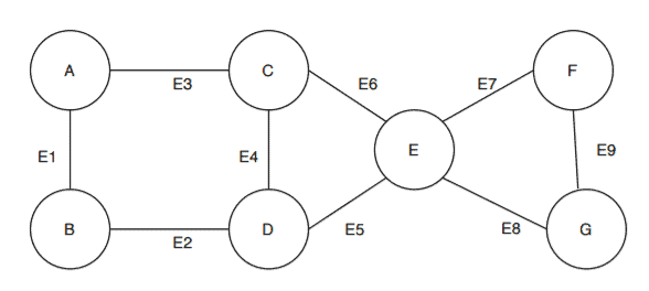
Here we’ve got a graph $G_1$ with a vertex set $V = (A, B, C, D, E, F, G)$ and edge set $E = (E_1, E_2, E_3, E_4, E_5, E_6, E_7, E_8, E_9)$ . Let’s start with the vertex $A$ and see if removing it and its and associated edges will disconnect the graph.

In this case, removal of vertex $A$ and associated edges $E_1$ and $E_3$ doesn’t disconnect the graph. Therefore, $A$ isn’t an articulation point.

But now let’s try vertex $E$ and itss associated edges $E_5$ , $E_6$ , $E_7$ , $E_8$ . This divides the graph $G_1$ into two connected components:

The first component $C_1$ with vertex set $(F, G)$ and edge set $(E_9)$
The second component $C_2$ with vertex set $(A, B, C, D)$ and edge set $(E_1, E_2, E_3, E_4)$

Thus, removing $E$ satisfies the articular point definition. Therefore, vertex $\textbf{E}$ is an articulation point in $\mathbf{G_1}$ .

4. Algorithm to Find All Articulation Points

In this section, we’ll present an algorithm that can find all the articulation points in a given graph.

This is a Depth First Search (DFS) based algorithm to find all the articulation points in a graph. Given a graph, the algorithm first constructs a DFS tree.

Initially, the algorithm chooses any random vertex to start the algorithm and marks its status as visited. The next step is to calculate the depth of the selected vertex. The depth of each vertex is the order in which they are visited.

Next, we need to calculate the lowest discovery number. This is equal to the depth of the vertex reachable from any vertex by considering one back edge in the DFS tree. An edge $(X, Y)$ is a back edge if $Y$ is an ancestor of edge $X$ but not part of the DFS tree. But the edge $(X, Y)$ is a part of the original graph.

After calculating the depth and lowest discovery number for the first picked vertex, the algorithm then searches for its adjacent vertices. It checks whether the adjacent vertices are already visited or not. If not, then the algorithm marks it as the current vertex and calculates its depth and lowest discovery number.

After calculating the depth and lowest discovery number for all the vertices, the algorithms take a pair of vertices and checks whether its an articulation point or not. Let’s take two vertices $V_1$ and $V_2$ . We’re further considering $V_1$ is a parent, and $V_2$ is a child vertex. If the lowest discovery number of $V_2$ is greater than or equal to the depth of $V_1$ , then $V_1$ is an articulation point.

There’s one special case when the root is an articulation point. The root is an articulation point if and only if it has more then one child in the tree. That’s why we put a checking condition in our algorithm to identify the root of the tree.

5. Running the Algorithm on a Graph

In this section, we’ll take a graph and run the algorithm on the graph $G_2$ to find out the articulation points:

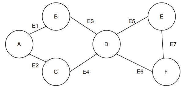
Now we’ll convert the graph $G_2$ to a DFS tree. We’ll start from a vertex and construct the tree as we visit the vertices:

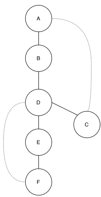
In this case, we started with the vertex $A$ and then visited the vertices $B, D, E, F$ . After the vertex $F$ , we go back and check if there is any vertex adjacent to $E$ , which there isn’t.

Similarly, we check for $D$ . Vertex $D$ has the adjacent vertex $C$ , which is not included in the tree. So we include vertex $C$ . At this point, we’re done with the construction of the DFS tree.

Notice that there are two dotted edges from vertices $F$ to $D$ and $C$ to $A$ . These are the back edges and are not part of the DFS tree.

Next, we’ll calculate the depth and lowest discovery number for all the vertices:

The depth number for each vertex is calculated as they are visited in the DFS tree. For example, vertex $A$ has a depth number $1$ and it denotes that the algorithm visits the vertex $A$ one the very first time in the DFS tree. Similarly, the depth number of vertex $B$ is $2$ . It depicts that the vertex $B$ is the second vertex the algorithm visited the DFS tree.

Let’s talk about how the algorithm calculates the lowest discovery number for each vertex. The rule is simple: Search the reachable vertices with the back edge and see in which vertex this back edge lands. The lowest discovery number of the current vertex will be equal to the depth of that vertex where the back edge lands.

Let’s say we want to calculate the lowest discovery number for vertex $B$ . The neighbor vertex is $D$ , but it doesn’t have any back edge. So the search goes on and reaches vertex $C$ . Vertex $C$ has a back edge, and it connects to vertex $A$ . The lowest discovery number of $B$ is equal to the depth of $A$ . Therefore the lowest discovery number of $B$ is $1$ .

We can calculate the lowest discovery number for all other vertices in the DFS tree in a similar way.

Now, to find the articulation points, we need to take a pair of vertices $(u, v)$ where $u$ is the parent of $v$ according to the DFS tree. Let’s start with a random pair of vertices $(E, F)$ where $E$ is the parent of $F$ .

Checking condition: $low[F] \geq depth[E] \implies 3 \geq 4 \implies FALSE$

Therefore, there is no articulation point here. Now let’s take another pair $(D, E)$ where $D$ is the parent of $E$ .

Checking condition: $low[E] \geq depth[D] \implies 3 \geq 3 \implies TRUE$
Checking condition 2: $D\ is\ not\ a\ root\ \Rightarrow TRUE$

Therefore, we can conclude that the vertex $D$ is an articulation point in the graph $G_2$ .

In this way, we can find out all the articulation points in any given graph.

6. Time Complexity Analysis

The algorithm mainly uses the DFS search with some additional steps. So basically, the time complexity of this algorithm is equal to the time complexity of the DFS algorithm.

In case the given graph uses the adjacency list, the time complexity of the DFS algorithm would be $\mathcal{O}(V + E)$ . Therefore, the overall time complexity of this algorithm is $\mathcal{O}\mathbf{(V + E)}$ .

7. Applications

The concept of articulation points is very crucial in a network. The presence of articulation points in a connected network is an indication of high risk and vulnerability. If a connected network has an articulation point, then a single point failure would disconnect the whole network.

In computer science, one popular problem is to find out the maximum amount of flow passing from a source vertex to a sink vertex. This problem is known as the max-flow min-cut theorem. The concept of articulation point is used here to find the solution.

8. Conclusion

In this tutorial, we’ve presented a DFS-based algorithm to find all the articulation points in a graph.

We also demonstrated an example to verify the algorithm and mentioned a couple of applications of articulation points.

Full Archive

About Baeldung

Core Concepts

Operating Systems

Artificial Intelligence

Graph Theory

Latex