Learn through the super-clean Baeldung Pro experience:
>> Membership and Baeldung Pro.
No ads, dark-mode and 6 months free of IntelliJ Idea Ultimate to start with.
Last updated: February 28, 2025

Learn through the super-clean Baeldung Pro experience:
>> Membership and Baeldung Pro.
No ads, dark-mode and 6 months free of IntelliJ Idea Ultimate to start with.
Gaussian Mixture Models (GMMs) are frequently used for clustering data, especially when the underlying data distribution is difficult to divide into distinct clusters.
In this tutorial, we’ll learn about Gaussian Mixture Models. However, let’s first start with the definition of clustering.
The machine learning technique of clustering groups related data points together into clusters. Clustering aims to identify patterns or structures in data without using labels or categories. In this regard, the algorithm discovers inherent patterns in the data without access to labelled samples, making it unsupervised learning.
We group or cluster data points in a dataset so that they are more similar to one another than those in other clusters, thereby achieving the purpose of clustering. Typically, we can expresses the similarities between data points in terms of specific characteristics or properties of the data.
Many different fields find uses for customer segmentation, picture segmentation, document categorization, anomaly detection, and other clustering. Therefore, it can help with data preparation, provide insights into the natural structure of the data, and help comprehend linkages within the data without prior knowledge of the ground truth labels.
Using Gaussian Mixture Models (GMMs), we group data points into clusters based on their probabilistic assignments to various Gaussian components. Let’s recall the flowchart for Gaussian Mixture Models:
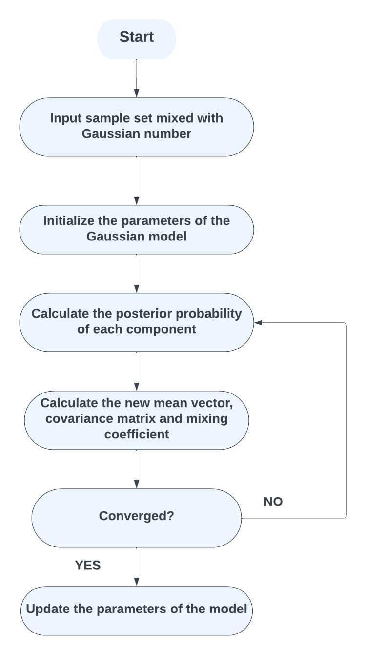
We’ll follow these steps to implement Gaussian Mixture Models.
We must ensure that the size and preprocess of the dataset are suitable before beginning. Techniques like principal component analysis might be used.
The user employs several clusters (Gaussian components) in the GMM. Methods like the Elbow Method, Silhouette Score, or Bayesian Information Criterion (BIC) can establish the ideal number of components.
Provide initial estimates for the means and covariance using methods like K-means clustering and initialize the Gaussian components’ means, covariance types, and mixing coefficients. There are three covariance types and we must choose depending on our data:
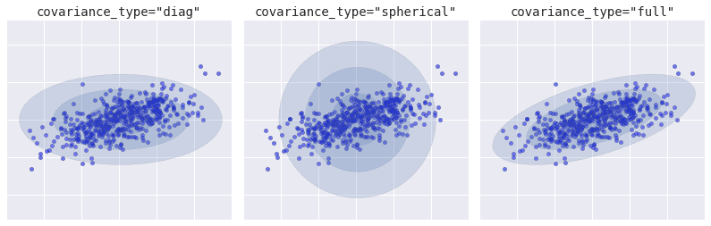
In K-means clustering, we have one option and it’s circular. Circular clusters might not be a good fit for all data clusters. However, we have the flexibility to choose different types of clusters in Gaussian Mixture Models.
Each data point’s likelihood to belong to each Gaussian component will be calculated as part of the E-Step (Expectation). Standardize these probabilities by determining the likelihood of each data point under each Gaussian distribution to determine responsibilities. We should determine the duties in the E-Step and update the M-Step parameters (means, covariance matrices, and mixing coefficients):
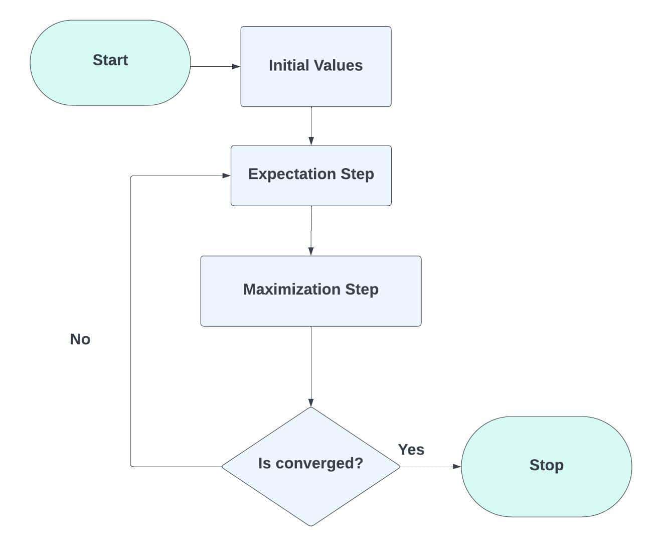
In this step 5, we must alternate between the E-step and M-step until convergence. When the change in log-likelihood or parameter estimations becomes insignificant between iterations, convergence has occurred.
The GMM should send each data point to the Gaussian component with the highest responsibility after it has been trained, assigning each data point a cluster.
In this context, let’s consider the following data:
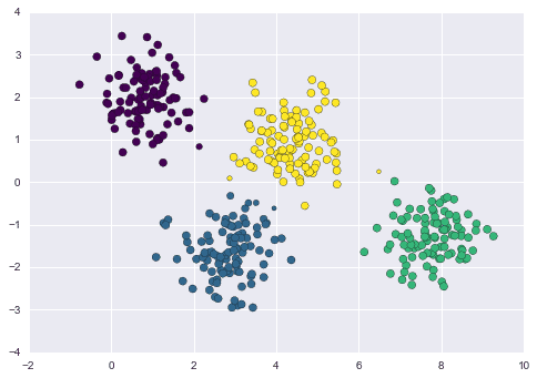 Let’s start with some guesses and then evaluate our results. In this case, the number of components is 4, the random state or seed is 42 and the covariance type is spherical:
As we can see here, our data can be grouped or clustered better. Therefore, we can prefer other types of covariances.
In this step, we’ll visualize the clusters by plotting the data points and the computed Gaussian components. We should utilize contour charts to show the density of each Gaussian component.
In this step, we’ll examine the resulting clusters. In order to do this, we must analyze each cluster’s properties in light of its matching Gaussian component’s mean and covariance.
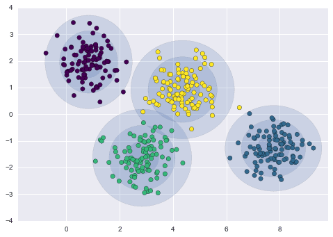
We can use external measures like silhouette score, adjusted Rand index or eye examination to assess the clustering quality since GMMs do not come with built-in metrics for measuring cluster quality. Let’s consider the following clustering examples. We’ll decide which fits our data best, circular or the other.
This is the circular (spherical) covariance type applied for the same data with the same parameters:
This is the elliptical or the full covariance type applied for the same data with the same parameters:
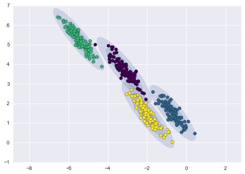
We can see that the elliptical covariance type fits our data better.
At this step, we’ll predict and assign new data if needed as we did in some parts of the previous steps.
Due to their non-convex nature, GMMs might be sensitive to initialization and might not always converge to the global optimum. GMMs frequently require careful parameter adjustment and initialization techniques to get effective clustering results.
Researchers have used Gaussian Mixture Models (GMMs) for clustering in various disciplines due to their adaptability in capturing complex data distributions. Let’s explore some examples of use cases in which GMMs can be applied for clustering effectively.
GMMs can divide images into areas or objects based on colour, texture, or other visual characteristics. Each Gaussian component can represent a different portion of the image.
We can use anomaly detection to find outliers or anomalies in a dataset using GMMs. Fraud detection, network security, and quality control can all benefit from anomalies, which are data points with low probabilities under the GMM.
We can use GMMs to group text documents according to their content or even categorize the land cover in satellite photos, assisting in disaster response, urban planning, and environmental monitoring.
GMMs can spot various market trends and regimes by analyzing financial time series data, and can also help with risk control and portfolio optimization.
We can group DNA sequences, gene expression profiles, and other biological data using GMMs. We can spot trends in gene function, disease classification, and medication development with clustering.
Groups can be divided according to their demographics, buying patterns, or other characteristics by companies utilizing GMMs. We can create individualized consumer experiences and target marketing campaigns.
Always remember that GMMs may not be ideal for all clustering tasks. Because they can be computationally expensive for large datasets and are sensitive to initialization and component number.
Several clustering applications benefit from the many benefits of Gaussian Mixture Models (GMMs). On the other hand, drawbacks and difficulties need to be considered when using Gaussian Mixture Models (GMMs) for clustering or other tasks, despite their numerous advantages.
| Pros | Cons |
|---|---|
| GMMs can capture clusters of varying sizes, forms, and orientations. K-means requires spherical clusters with equal variance, whereas GMMs support more variable covariance structures. They can accommodate clusters of elongated, rotated, or varied sizes. GMMs perform well in unsupervised learning tasks without labelled data points to direct the clustering process. | The EM algorithm may not scale well to large datasets due to GMMs’ iterative processing requirements. When working with high-dimensional or complex data distributions, the EM method can occasionally become trapped in local optima. |
| GMMs can produce new data that is consistent with the discovered distribution. This can generate synthetic data, enhance existing data, and do other generative activities. The Expectation-Maximization EM technique used for parameter estimation in GMMs assures convergence, even though it occasionally converges to the local optimum. This problem can be addressed by using different initialization techniques. | GMMs may be sensitive to outliers because they presume data points are produced from a Gaussian distribution. Therefore, outliers might significantly impact the predicted parameters. Given the cluster assignment, GMMs presume that each feature within a data point is independent. Henceforth, possibly not all forms of data will conform. |
| The clusters’ distributions of the data and their connections can be revealed by visualizing them as Gaussian distributions using GMMs. Cross-validation or the Bayesian Information Criterion BIC can help choose the best number of components and prevent overfitting or underfitting. | Determining the precise significance of the shape and orientation of a Gaussian component can be difficult when modelling many cluster shapes with GMMs.As the number of dimensions rises, the difficulty of estimating the covariance matrices increases due to more parameters to estimate. Thus, this may result in overfitting or problems with parameter estimates. |
| The soft assignment is a feature of GMMs, allowing each data point to belong to many clusters with various probabilities. Thus, this helps when data points are uncertain or lie between clusters. | GMMs continue to be a useful tool for a range of clustering tasks, particularly when the underlying data distribution is intricate and multimodal, despite these drawbacks. Consequently, consider whether these restrictions match the demands of our particular scenario before choosing to use GMMs or looking into other clustering strategies. |
Gaussian Mixture Models excel when the underlying data distribution is complex, multimodal, or ambiguous, making them flexible and strong clustering methods. A wide range of clustering applications can exploit their probabilistic nature and soft assignment.
Gaussian Mixture Models are a powerful and widely used statistical tool for clustering.
In this article, we learned about the definitions, implementation steps, use cases, advantages, and disadvantages of Gaussian Mixture Models for clustering.