Yes, we're now running our only Summer Sale. All Courses are 30% off until 20th July, 2026:
Fuzzy Search Algorithm for Approximate String Matching
Last updated: June 8, 2023

Learn through the super-clean Baeldung Pro experience:
>> Membership and Baeldung Pro.
No ads, dark-mode and 6 months free of IntelliJ Idea Ultimate to start with.
1. Introduction
There are various optimization algorithms in computer science, and the Fuzzy search algorithm for approximate string matching is one of them.
In this tutorial, we’ll look at what this fuzzy matching means and what it does. Then, we’ll go through different types and applications of fuzzy matching algorithms.
Finally, we’ll choose an example to demonstrate the solution to an approximate string matching issue.
2. What Is Fuzzy Matching?
Fuzzy Matching or Approximate String Matching is among the most discussed issues in computer science. In addition, it is a method that offers an improved ability to identify two elements of text, strings, or entries that are approximately similar but are not precisely the same.
In other words, a fuzzy method may be applied when an exact match is not found for phrases or sentences on a database. Indeed, this method attempts to find a match greater than the application-defined match percentage threshold.
3. Applications of Fuzzy Matching
We can find fuzzy searches in different applications. This technique search resolves the complexities of spelling in all languages, rushed-for-time typers, and clumsy fingers. Fuzzy searches are also used to gather user-generated data. This is usually unreliable because users misspell the same word or use localized spelling. Also, this includes sound and phonetics-based matching.
Moreover, common applications of approximate matching include matching nucleotide sequences in front of the availability of large amounts of DNA data. In addition, we can use approximate matching in spam filtering and record linkage here records from two disparate databases are matched.
4. Algorithms Used for Fuzzy Matching
We cover here some of the important string matching algorithms:
4.1. Naive Algorithm
Among the several pattern search algorithms, naive pattern searching is the most basic. It looks for all of the main string’s characters in the pattern. Precise string matching (identifying one or all exact instances of a pattern in a text) presents the naive approach. Most importantly, there are no pre-processing steps required. By testing for the string once, we can find the substring. Also, it takes up no more space to carry out the process.
4.2. Hamming Distance Algorithm
The Hamming distance is a mathematical concept used in computer science in different fields such as signal processing and telecommunications. This plays an important role in the algebraic theory of code modification. In fact, it allows quantifying the difference between the two sequences of symbols. In the case of two strings, the Hamming distance designates the number of positions at which the corresponding character is different.
4.3. Levenstein Distance Algorithm
In computer science, the Levenstein Distance method allows to measure the similtarity between the source string  and the target string
  . The distance between and presents the number of insertions, substitutions, and deletions. For example:
- If is “test” and t corresponds “test”, so,
 , since no transformations are required. The strings are already identical
 - If is “test” and t corresponds “tent”, so,
 , because we have one substitution (change to
  ) is adequate to modify into
4.4. N-gram Algorithm
An n-gram is a continuous series of elements from a well-defined text or audio sequence. We can show the objects as syllables, phonemes, words, characters, or base pairs, depending on the application. A probabilistic language model, or n-gram model, is a sort of probabilistic language model. In the form of a  –order Markov model, it is possible to forecast the next item in such a sequence.
4.5. BK Tree Algorithm
A BK tree is a type of metric tree that is tailored to discrete metric spaces. To better understand, we can consider the integer discrete metric  . Then, BK-tree is defined as follows. An arbitrary element
  is chosen as the root node. The root node can reach zero or more subtrees. The
  subtree is formed recursively from all elements
  such that
  . We use BK-trees for approximate matching of strings in a dictionary.
4.6. Bitap Algorithm
The Bitap algorithm is an approximate string matching algorithm. The algorithm indicates whether a given text contains a substring “approximately equal” to a given pattern, where approximate equality arises in terms of Levenshtein distance.
Indeed, if the pattern and the substring are at a given distance k from each other, then the algorithm considers them equal. The advantage of this algorithm over other methods is its use of bitwise operations. This makes it very fast.
5. Fuzzy Matching Algorithm Example
In this part, we choose to describe the Naive pattern searching algorithm. It checks for all characters of the main string to the pattern. Certainly, using the Naive algorithm, we can find one or all of the same pattern occurrences in a text. In fact, we can discover substring by checking once for the string.
5.1. Algorithm
So, we can see here the pseudocode of the fuzzy matching algorithm:
algorithm NaiveStringMatcher(t, p):
    // INPUT
    //    t = the text to search within
    //    p = the pattern to search for
    // OUTPUT
    //    Prints the positions where the pattern occurs in the text

    n <- t.length
    m <- p.length

    for s <- 0 to n - m:
        if p[1 : m] = t[s + 1 : s + m]:
            print "Pattern occurs with shift" s
Firstly, the naïve approach tests all the possible placement of pattern ![p [1...m]](/wp-content/ql-cache/quicklatex.com-278e01f92382b5cdbf66ba7e4aaf1271_l3.svg "Rendered by QuickLaTeX.com") relative to text
relative to text ![t [1...n]](/wp-content/ql-cache/quicklatex.com-c7fd6f12bd711598ca035dae19f6d6e0_l3.svg "Rendered by QuickLaTeX.com") . Then, we try shift
. Then, we try shift  , successively and for each shift . Finally, we compare
 ![t [s+1...s+m]](/wp-content/ql-cache/quicklatex.com-b8da502f4264a56879232f016e2572b6_l3.svg "Rendered by QuickLaTeX.com") to . The main efficiency of this algorithm is that the valuable information gained about the text for one shift is totally ignored when considering other shifts of .
to . The main efficiency of this algorithm is that the valuable information gained about the text for one shift is totally ignored when considering other shifts of .
5.2. Example of Fuzzy Searching Algorithm
Here we can see how the algorithm works in more detail. In fact, we choose an example of the naïve pattern search approach.
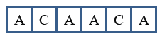
We define  as the text and
  as the pattern, with
  and
and  .
.
The text :
The pattern :
Using the naïve method, we have to find all the positions where this occurs in the text .
Firstly, we start comparing text and pattern:
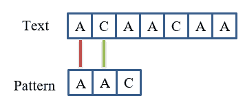
As a result, the first character matches: ![P[0]==T[0]](/wp-content/ql-cache/quicklatex.com-348d153faa42ae65cbb07b52f915dc9a_l3.svg "Rendered by QuickLaTeX.com") and the second character doesn’t matches:
and the second character doesn’t matches: ![P[1] \ne T[1]](/wp-content/ql-cache/quicklatex.com-b1c54f99e151148ecf9d2a6d0d6ac09a_l3.svg "Rendered by QuickLaTeX.com") .
.
Secondly, we must check the first character of with the second character of as shown in this figure:
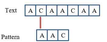
So, we have ![P[0] \ne T[1]](/wp-content/ql-cache/quicklatex.com-41400cc8237eb14651986546ab2f82a4_l3.svg "Rendered by QuickLaTeX.com") .
.
Then, we check the pattern from ![T[2]](/wp-content/ql-cache/quicklatex.com-6ee04dbdd29867d224b1c7cdb76b8a61_l3.svg "Rendered by QuickLaTeX.com") .
.
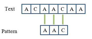
As a result, we obtain ![P[0]==T[2]](/wp-content/ql-cache/quicklatex.com-b21dabdd105bf326e1709c4755c538bc_l3.svg "Rendered by QuickLaTeX.com") . While verifying the next characters, we get
. While verifying the next characters, we get ![P[1]==T[3]](/wp-content/ql-cache/quicklatex.com-c82e86c7c58a027499ff8ac45543aeca_l3.svg "Rendered by QuickLaTeX.com") , and
, and ![P[2]==T[4]](/wp-content/ql-cache/quicklatex.com-9b9ff633fe4339e757421bc03e6ed5c7_l3.svg "Rendered by QuickLaTeX.com") .
.
Now, we will further check for the next occurrence of pattern as shown in the following figure:
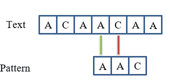
The result obtained is the following: ![P[0]==T[3]](/wp-content/ql-cache/quicklatex.com-4008a99df52c596f62c2f130896e3040_l3.svg "Rendered by QuickLaTeX.com") and
and ![P[1] \ne T[4]](/wp-content/ql-cache/quicklatex.com-1c66284bc32b749c3feb45910184b601_l3.svg "Rendered by QuickLaTeX.com") .
.
Consequently, we will not go further because there is no character left in the text of pattern to match.
6. Conclusion
In this article, we discussed the different techniques and applications of fuzzy matching algorithms. We have used the naïve method as a common algorithm to find approximate substring matches inside a given string. We introduced this algorithm because it’s highly effective and fast in solving approximate string matching issues.