How To Find a List of Possible Words From a Letter Matrix

1. Overview

In this tutorial, we’ll talk about the problem of finding the list of all possible words from a 2D letter matrix.

First, we’ll define the problem and get words in a 2D letter matrix. Then, we’ll give an example to explain it. Finally, we’ll present two different approaches to solving this problem and work through their implementations and time complexity.

2. Defining the Problem

Suppose we have a 2D letter matrix $M$ , and we were asked to generate all possible words that we can get from that matrix $M$ .

Initially, a word could be presented by a path in a 2D matrix, where we start from a cell that contains the first letter of the given word and look for the second letter in the eight adjacent cells of the current one. We keep moving until we reach the end of the word. In the end, the route that we take to get the word should have distinct positions (we can’t use the same cell more than once).

Let’s take a look at the following example. Given the following 2D letter matrix:

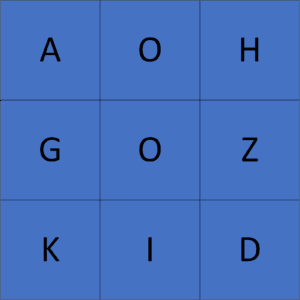
We could get multiple valid words like $Good$ , $God$ , $Dog$ , $Kid$ , etc. For example, let’s take a look at how to get the word $Good$ from the previous matrix:

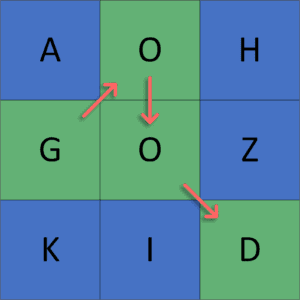
As we can see, we get the word $Good$ by taking a sequence of adjacent cells and not taking the same cell twice. Finally, the result of the previous example will be a list of all possible valid words that could be formed from the given 2D matrix.

3. Naive Approach

3.1. Main Idea

The main idea in this approach is to try all the possible paths in the given matrix. We’ll check whether each path creates a valid word or not.

First, we have a dictionary of words that will define whether a word is valid or not. Second, we run a backtracking method for each cell of the given matrix that generates all the possible paths in the given matrix that start at the current cell.

Next, each time we reach a cell, we append it to the current path and mark it as a visited cell to not consider it again. Then, we check whether it forms a valid word for every path. If so, we append it to the set of possible words that could be generated from the given matrix. Otherwise, we ignore it and check other paths.

Finally, we get a list of all the possible valid words generated from the given matrix $M$ .

3.2. Algorithm

Let’s take a look at the implementation of the algorithm:

Initially, we declare the $backtrack$ function to generate all possible valid words in the given matrix $M$ . The function will have four parameters. $x$ and $y$ represent the current position in the given matrix $M$ , $word$ represents the current word that we have until now, and $possible\_ words$ represents all possible valid words that we generated from the given matrix $M$ .

First, we append the letter at the current cell to $word$ , and we mark the current cell as visited. Next, we iterate over all the possible valid words in the dictionary to check whether the current word is valid or not. If we find a match, we append $word$ to the set of $possible\_ words$ .

Second, we declare a transition array to move to the eight adjacent neighbor cells. For each one, we check if it’s in the boundary of the given matrix and not visited yet, then we move to it and call the $backtrack$ function at it.

Finally, we backtrack on the current cell’s character and mark it as unvisited, so we can use it in the future.

We run the $backtrack$ function starting from each cell of the given matrix, and the $possible\_ words$ set will have all possible valid words that could be generated from that cell. Combining these sets will provide us with all the words generated from the given 2D letter matrix.

3.3. Complexity

The time complexity of this algorithm is $\boldsymbol{O(8^N \times M)}$ , where $N$ is the number of cells in the given matrix and $M$ is the sum of the length of all words in the dictionary. The reason behind this complexity is that for each cell, we have $8$ different possibilities for the next cell, and for each possibility, we iterate over all the valid words in the dictionary to check for a match with the current word.

If the function is called from each cell inside the grid, then the complexity will be $\boldsymbol{O(X \times Y \times 8^N \times M)}$ , where $\boldsymbol{X}$ and $\boldsymbol{Y}$ are the number of rows and columns in the matrix $\boldsymbol{M}$ .

4. Trie Approach

4.1. Main Idea

The main idea in this approach is the same as the previous one, but we optimize the complexity of matching the current word with a word from the dictionary using the trie data structure.

First, we’ll create a trie data structure containing all the dictionary words to check if a word is valid in constant time. Second, we’ll run a backtrack function from each cell and generate all the possible words that start at that cell.

Next, for each cell, we’ll check if the current word we have is inside our trie structure or not. If so, we append it to the set of possible words. Then, we try to move to a non-visited adjacent cell to search for any other valid words.

Finally, the possible words set will have all the words that could be generated from the given matrix.

4.2. Building Trie Structure

Let’s take a look at the implementation of creating a trie structure from a dictionary:

We declare the $BuildTrie$ function that will create a trie structure containing all the words of the dictionary, this function will take one parameter $dictionary$ , which represents a list of all possible valid words in the language.

Initially, we declare the $root$ of the trie structure that will store all the words of the given dictionary. Then, we iterate over each word in the dictionary and insert it in our trie structure.

Finally, we return the $root$ of the trie structure that contains all the words of the dictionary.

4.3. Algorithm

Let’s take a look at the implementation of the algorithm:

Initially, we have the same $backtrack$ function as before with an additional one parameter $trie$ , which represents the root of the trie structure that has all the possible valid words.

First, we check if the current character is not one of the children of the current node in the trie structure, which means we can’t take the current character. So, we return and break out of the backtrack function. Otherwise, we move to the child of the $trie$ , which has the current character.

Second, we’ll do the same process as the previous approach. However, to check the validity of the current word, we’ll use the trie structure to check if the current word is valid or not in constant time.

After that, we call the $backtrack$ function on all the eight adjacent cells.

Finally, the $possible\_ words$ set will have all possible valid words that could be generated from the starting position. Calling this function from each cell will give us the list of all possible words.

4.4. Complexity

The time complexity of this algorithm is $\boldsymbol{O(8^N + M)}$ , where $N$ is the number of cells in the given matrix and $M$ is the sum of the length of all words in the dictionary. The reason behind this complexity is the same as the previous approach but instead of iterating over all the possible words in the dictionary, we check the current word in constant time using a trie data structure that we’ll build in $O(M)$ time complexity.

If the function is called from each cell inside the grid, then the complexity will be $\boldsymbol{O(X \times Y \times (8^N + M))}$ , where $\boldsymbol{X}$ and $\boldsymbol{Y}$ are the number of rows and columns in the matrix $\boldsymbol{M}$ .

5. Conclusion

In this article, we discussed the problem of finding all the possible words from a 2D letter matrix. First, we provided an example to explain the problem. Then, we explored two different approaches, each with better time complexity.

Finally, we walked through their implementations and explained the idea behind each of them.

Full Archive

About Baeldung

Core Concepts

Operating Systems

Artificial Intelligence

Graph Theory

Latex