

Learn through the super-clean Baeldung Pro experience:
>> Membership and Baeldung Pro.
No ads, dark-mode and 6 months free of IntelliJ Idea Ultimate to start with.
Learn through the super-clean Baeldung Pro experience:
>> Membership and Baeldung Pro.
No ads, dark-mode and 6 months free of IntelliJ Idea Ultimate to start with.
In this tutorial, we’ll present Expectimax, an adversarial search algorithm suitable for playing non-deterministic games.
In particular, we’ll focus on stochastic two-player games, which include random elements, such as the throwing of dice. However, since Expectimax is a modification of Minimax, the algorithm for playing deterministic games, we’ll first introduce the latter.
In classical search, an AI agent looks for the optimal sequence of actions to achieve some goal. The agent is the only entity in its environment that can take action, so all the changes come through its actions. Since it’s the only one there, the agent models only its state of belief about the environment. Then, the sequence of actions becomes a path between the states.
In adversarial search, the agent still searches for the optimal sequence of actions, but the environment is different. In contrast to classical search, it’s not alone here. There is at least one other AI (or human) agent that can act in their shared environment. Furthermore, the agents have conflicting goals, so they compete with one another. So, the optimal sequence the agents want to find is the one that leads to victory over the opponents.
The agents, therefore, model not only their states but also the states of all the other agents they compete with. Good examples of adversarial search are two-player or multiplayer games such as chess and poker.
In AI game playing, we often refer to the states as positions and actions as moves. Just as it’s the case with general problems in classical search, the definition of a game includes multiple components:
 : it specifies the initial state of the game before the very first move
 : a function that tells us which player (agent) is to make its move in the state
 : a function returning all the moves legal in the state
  : the transition model specifying which state we get in by applying action
  in the state
  : a function that identifies the states in which the game is over
 : the utility function assigning a numerical value to player
  in terminal state
 This article will focus on the games in which the utilities for all the players in each terminal state sum up to a constant. That constant is 0 most of the time, which is why we call such games “zero-sum”, although “constant-sum games” would be a more precise term. So, the players try to win the game by maximizing their utility at the end of it.
In deterministic games, there is no uncertainty about the environment, the actions possible to take in a state, and the state we get after applying an action. Therefore, all the components in the game definition are completely deterministic.
For instance, tic-tac-toe is a deterministic game. For any board state, we know without any doubt whose turn it is to play, which cells the player can mark, and what the board will look like after each possible move.
To play two-player games that are both deterministic and zero-sum, we use the algorithm known as Minimax.
The two players go by names MAX and MIN. MAX is the player our AI agent runs Minimax for, while MIN is the opponent. MAX chooses the moves to maximize its utility, whereas MIN tries to minimize the result of MAX. Since the game is zero-sum, MIN maximizes its utility by minimizing that of MAX.
The search tree starts in the current state (which is initially) and branches out by all the possible move sequences. A node  in the tree points to the state the agent gets to by following the path of moves from
  to .
to .
So, similar to classical search, a node  is a structure representing a path to its state
  and contains a pointer to its parent (
 ). But, to keep things simple, we’ll consider that the functions
  through
  in the game definition in Section 3 operate on nodes as well.
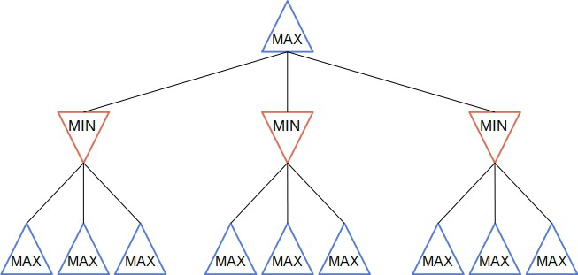
Minimax explores the tree by simulating the game and calculating the minimax value of each node:
Starting from the node when it’s the MAX’s turn to play, Minimax chooses the move which leads to the child with the highest minimax value. Let’s say that  is that child. Then, MIN makes its move by running its instance of Minimax on , minimizing the utility of MAX. After that, it’s again MAX’s turn to make a move, so it starts from , and so on:
This is the pseudocode of Minimax:
algorithm Minimax(game_description, u, player):
    // INPUT
    //    game_description = description of the game
    //    u = the node
    //    player = the player to act as MAX
    // OUTPUT
    //    The optimal move for player in node u's state

    (move, value) <- MAXVALUE(u, player)

    return move

function MAXVALUE(u, player):
    // INPUT
    //    u = the node
    //    player = the player to act as MAX
    // OUTPUT
    //    The best move and its value

    if terminal(u):
        return (null, utility(u, player))

    (best_move, max_value) <- (null, -infinity)

    for max_move in moves(u):
        (min_move, value) <- MINVALUE(result(u, max_move), player)
        if value > max_value:
            (best_move, max_value) <- (max_move, value)

    return (best_move, max_value)

function MINVALUE(u, player):
    // INPUT
    //    u = the node
    //    player = the player to act as MAX
    // OUTPUT
    //    The best move and its value

    if terminal(u):
        return (null, utility(u, player))

    (best_move, min_value) <- (null, +infinity)

    for min_move in moves(u):
        (max_move, value) <- MAXVALUE(result(u, min_move), player)
        if value < min_value:
            (best_move, min_value) <- (max_move, value)

    return (best_move, min_value)
So, Minimax traverses the whole game tree to the leaves and returns the best move for the player at hand. If the tree is too deep, we cut off the search at some depth, making non-terminal nodes our new leaves. Then, we evaluate the leaves by estimating their minimax value instead of calculating the utilities of the actual leaves and propagating them upward. We can also prune the tree with the alpha-beta search.
Evaluation functions we use for estimation should return numeric values that correlate with the actual minimax values. They should also be computationally lightweight and easy to implement. But, if it’s hard to design a quality evaluation function, we can use Monte Carlo Tree Search (MCTS) to evaluate a node.
Unlike deterministic games, the stochastic ones have at least one probabilistic element. For example, may return different sets of legal actions each time we call it, depending on the outcome of some random event such as the throwing of dice. Or, the result of an action can lead to multiple states, each with a certain probability.
For instance, we roll dice in a game of backgammon before each move. The numbers we get determine what moves we can make. MAX doesn’t know in advance what moves it will choose from at any point in the game, and the same goes for MIN’s actions. All the AI agent has at those chance branching points is a probability distribution over possible moves.
So, the search tree of stochastic games has an additional node type: the chance nodes. A chance node represents a probability distribution over the set of moves available to the player whose node is the parent of :
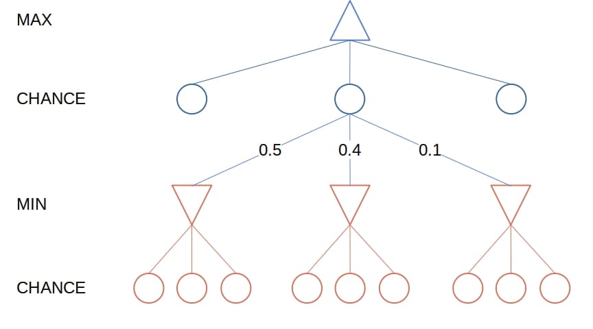
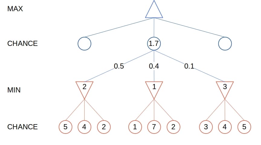
Instead of the minimax values, the nodes have the expectimax values. They’re the same as the minimax values for MIN and MAX nodes, but for a chance node, the expectimax value is the expected value of its children:
Or, as a recurrence:
 is an outcome of the random event at chance nodes, and
  is its probability.
The ExpectiMax algorithm is very similar to MiniMax:
algorithm Expectimax(u, player):
    // INPUT
    //    u = a node representing the current state of the game
    //    player = the player to act as MAX
    // OUTPUT
    //    The optimal move for player in node u's state

    (move, value) <- EXPECTIMAX_VALUE(u, player)
    return move

function EXPECTIMAX_VALUE(u, player):
    // INPUT
    //    u = a node representing the current state of the game
    //    player = the player to act as MAX
    // OUTPUT
    //    The expected value for the node u

    if u is a chance node:
        expected <- 0
        for r in moves(u):
            (move, value) <- EXPECTIMAX_VALUE(result(u, r), player)
            expected <- expected + P(r) * value
        return (null, expected)
    else if turn(u) = player:
        return MAX_VALUE(u, player)
    else:
        // this is a MIN node
        return MIN_VALUE(u, player)
Still, we should note two things. The first one is that the functions  and
and  don’t call one another like they do in Minimax. Instead, both call
  .
.
The second thing is that if is a chance node, then there isn’t a single move to return. Its expectimax value is the expectation over the outcomes of all the possible moves. We pair it with  , the empty move, for consistency with other cases.
Similar to what we did with Minimax trees, we’ll most probably have to limit the depth of the Expectimax trees by cutting off the search at some point. However, we’ll have to pay special care to design the evaluation functions that estimate non-terminal leaf nodes.
The evaluation functions in Minimax need only be correlated with the probabilities of winning. More precisely, they should preserve the order of moves. For example, let move  lead to state
  in which the player has
  chance to win, and let
  lead to the state
  where the probability is
  . Then, Minimax requires only that evaluation function
  assigns a higher value to :
  so that
  can use it to win.
However, in Expectimax, the evaluation function should be a positive linear transformation of the probabilities of winning. Thus, even if the order remains the same, small changes to the evaluation values can lead the agent to choose a different move.
If designing a good evaluation function proves to be too challenging, we can opt for MCTS.
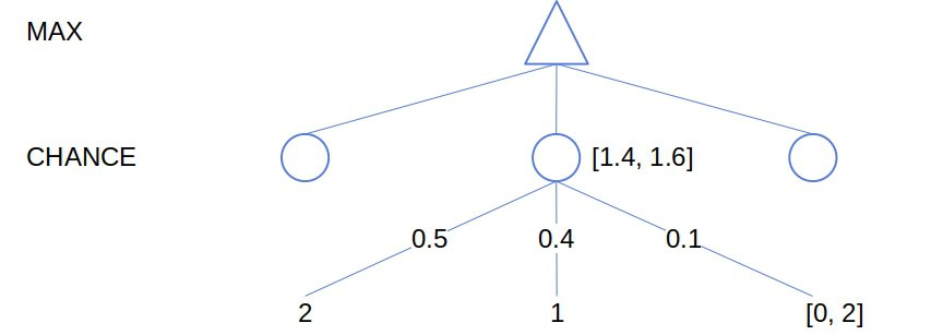
We can apply the alpha-beta pruning technique to Expectimax even though it may come as counter-intuitive at first sight. The goal of pruning is to prove that we don’t need to consider certain moves so that we completely disregard the sub-trees rooted in the nodes those moves lead us to. However, the expectimax values require visiting all the children of a chance node and calculating their expectimax values. So, it appears that pruning is incompatible with Expectimax.
But, there’s a way to circumvent this issue. If we bound the range of the evaluation function from below and above, we can determine the bounds of the expectimax value of a chance node even if we don’t evaluate all its children and their sub-trees:
In this article, we presented the Expectimax algorithm for stochastic games. We derived it from Minimax and talked about two optimization strategies: limiting the game tree depth and pruning the search tree.
![\[minimax(u) = \begin{cases} utility(u, \mathrm{MAX}),& \text{if } terminal(u) = true\\ \max_{a \in moves(u)} minimax(result(u, a)),& \text{if } turn(u) = \mathrm{MAX} \\ \min_{a \in moves(u)} minimax(result(u, a)),& \text{if } turn(u) = \mathrm{MIN} \end{cases}\]](/wp-content/ql-cache/quicklatex.com-23e78b4d17c29bab23dc19ec60fcb6ed_l3.svg "Rendered by QuickLaTeX.com")
![\[expectimax(u) = \begin{cases} utility(u, \mathrm{MAX}),& \text{if } terminal(u) = true\\ \max_{a \in moves(u)} expectimax(result(u, a)),& \text{if } turn(u) = \mathrm{MAX} \\ \min_{a \in moves(u)} expectimax(result(u, a)),& \text{if } turn(u) = \mathrm{MIN} \\ \sum_{r \in moves(u)} P(r)\cdot expectimax(result(u, r)), & \text{if } turn(u) = \mathrm{CHANCE} \end{cases}\]](/wp-content/ql-cache/quicklatex.com-a9f6efdb15164033a633e377e6c3b6a5_l3.svg "Rendered by QuickLaTeX.com")