Dragonfly Algorithm | Baeldung on Computer Science

1. Introduction

The Dragonfly Algorithm is one of the most recently developed heuristic optimization techniques. Moreover, it has shown its ability to optimize different real-world problems. In this tutorial, we’ll talk about the Dragonfly Algorithm and present the different steps of the algorithm.

2. What Is the Dragonfly Algorithm?

Mirjalili created the Dragonfly Algorithm at Griffith University in 2016. The Dragonfly Algorithm was inspired by the static and dynamic swarming behavior of dragonflies in the wild. In fact, the two required phases of optimization, exploration and exploitation, are represented by the static and dynamic swarming behaviors.

Also, dragonflies form sub-swarms and fly over different areas in a static swarm. This is similar to exploration, and it aids the algorithm in locating appropriate search space locations. On the other hand, dragonflies in a dynamic swarm fly in a larger swarm and in the same direction. In addition, this type of swarming is the same as using an algorithm to assist it converges to the global best solution.

3. Dragonfly Algorithm Steps

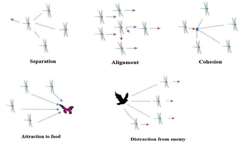
Generally, the behavior of swarms of the Dragonfly Algorithm follows three primitive principles:

Separation: which indicates the avoidance of neighboring static collisions
Alignment: which returns the speed of individuals paired with neighboring individuals
Cohesion: which indicates the individual tendency toward the center of the herd

Since the ultimate purpose of any swarm is to survive, all of the members should be drawn to food sources and away from potential attackers. So, there are five primary aspects in position updating of individuals in swarms when considering these two behaviors: Separation, Alignment, Cohesion, Attraction, and Distraction as shown in the figure below:

4. Dragonfly Algorithm Mathematical Model

As we mentioned in the previous section, the positioning movement of dragonflies consists of the following five behaviors. So, let’s define the operations:

4.1. Separation

We can calculate the Separation between two adjacent dragonflies as follows:

${S_i}={-\sum_{j=1}^N X}- {X_j}$ (1)

where ${X}$ presents the position of the current individual, $j^{(th)}$ indicates the neighboring individual and ${N}$ is the number of neighboring individuals.

4.2. Alignment

The equation is used to determine the alignment of dragonflies:

${A_i}=\frac{\sum_{j=1}^N V_j}{N}$ (2)

where ${V_j}$ describes the velocity of $j^{(th)}$ neighboring individual.

4.3. Cohesion

We can derive the Cohesion as follows:

${C_i}=\frac{\sum_{j=1}^N X_j}{N}-{X}$ (3)

where ${X}$ shows the position of the current individual, $j^{(th)}$ indicates the neighboring individual, and ${N}$ is the number of neighboring individuals.

4.4. Attraction

We compute the Attraction operation toward the source of food using this equation:

${F_i}={X^+} - {X}$ (4)

Where ${X}$ presents the position of the current individual, and ${X^+}$ describes the position of the food source.

4.5. Distraction

We can determine the Distraction from the enemy as shown here :

${R_i}={X^-} - {X}$ (5)

Where ${X}$ , shows the position of the current individual and ${X^-}$ denotes the natural enemy.

To update the position of artificial dragonflies in a search space and replicate their motions, two vectors are considered: step vector ( $\Delta X$ ) and position vector ( $X$ ).

So, the step vector presents the direction of the movement of the dragonflies. We can define this vector by the equation :

$\Delta {X_t+1}=(s {S_i}+ a {A_i}+c {C_i}+f {F_i}+r {R_i})+w \Delta {X_t}$ (6)

where $s$ , $a$ , $c$ , and $f$ are weights for the phases: separation, alignment, cohesion, attraction, and distraction. Also, $w$ presents the inertia weight, and $t$ is the iteration counter.

Exploration and exploitation stages can be achieved by changing the values of these weights.

The position vector is easily determined with the help of the step vector, as shown in the equation :

${X_t+1}= {X_t} + \Delta {X_t+1}$ (7)

In fact, low cohesion weight ( $c$ ) and high alignment weight ( $a$ ) are allocated to the exploration phase. Similarly, low alignment weight ( $a$ ) and high cohesion weight ( $c$ ) are assigned to the exploitation phase.

The position vector indicates the dragonfly’s location; however, if no surrounding solutions exist, the dragonflies must fly in a random search space, and their position must be updated using the adjusted equation :

${X_t+1}= {X_t} + {X_t}.levy(d)$ (8)

where $levy(d)$ is:

$levy(d)=0.01 \frac{{r_1}. {\sigma}}{|r_2|^{\frac{1}{\beta}}}$ (9)

where we range $r_1$ , $r_2$ in [0,1], $\beta$ is constant,

$\sigma$ is defined as follows:

$\sigma=(\frac{(\beta! \times sin (\frac{\pi\beta}{2}))}{(\frac{\beta-1}{2})!\times\beta\times 2^(\frac{\beta-1}{2})})^\frac{1}{\beta}$ (10)

5. Pseudocode of the Dragonfly Algorithm

Let’s now take a look at the different steps of the algorithm:

The Algorithm begins the optimization process by randomly producing a set of solutions to given optimization problems. To initialize the position and step vectors of dragonflies, random values defined within the lower and higher ranges of the variables are employed.

Each dragonfly’s position and step were updated in each cycle. In addition, the neighborhood of each dragonfly is picked for updating $(X)$ and $(Delta X)$ vectors by computing the Euclidean distance between all dragonflies and picking N of them. Then, we continued the position updating process iteratively until the end criterion was satisfied.

6. Example

We show here one specific example of a dragonfly’s behavior to better understand this method. This figure shows an example of dragonfly swarming behavior with increasing neighborhood radius using the previous mathematical model:

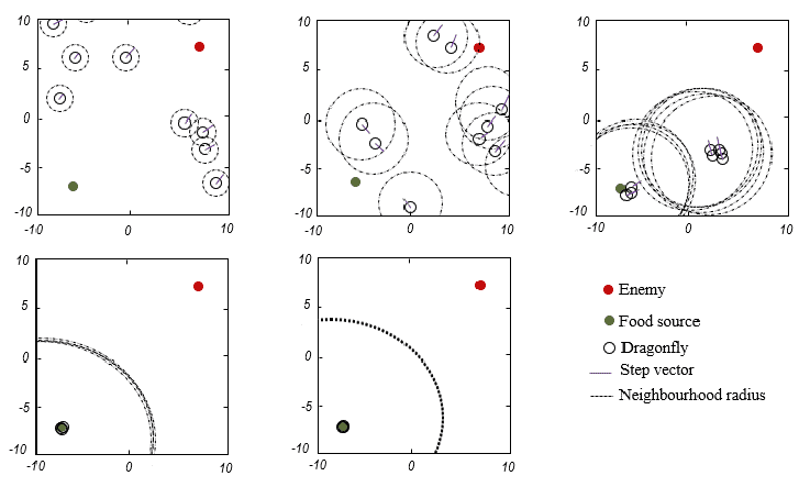
Indeed, different explorative and exploitative behaviors may be created during optimization using separation, alignment, cohesion, food, and enemy factors (s, a, c, f, r and w). Because the neighbors of dragonflies are so crucial, each dragonfly is supposed to have a neighborhood with a specific radius.

We utilize s= $0.1$ , a= $0.1$ , c= $0.7$ , f= $1$ , r= $1$ , and w is linearly decreased from $0.9$ to $0.2$ and with the parameters, we were able to stimulate different swarming behavior. Also, the green circle is a food source, black circles are individuals, the red circle indicates the enemy, and purple lines are the step vector of the dragonflies.

In fact, this image demonstrates how the suggested model moves individuals throughout the search area in relation to each other as well, food source, and enemy.

7. Conclusion

Generally, the Dragonfly Algorithm in applied science is offered in the following area: networking, machine learning, image processing, and wireless. Indeed, in this tutorial, we presented the Dragonfly Algorithm by describing its different steps and the mathematical model.

Full Archive

About Baeldung

Core Concepts

Operating Systems

Artificial Intelligence

Graph Theory

Latex