

Yes, we're now running our only Summer Sale. All Courses are 30% off until 20th July, 2026:
Learn through the super-clean Baeldung Pro experience:
>> Membership and Baeldung Pro.
No ads, dark-mode and 6 months free of IntelliJ Idea Ultimate to start with.
1. Introduction
In this tutorial, we’ll cover the Disjoint Set Union (DSU) data structure, which is also called the Union-Find data structure. Initially, we have a universe  of
of  elements:
  , and we’re interested in separating elements into independent (non-intersecting) sets. Additionally, we must support the union operation of two sets. Lastly, for any given element, we must be able to find the set it belongs to.
2. DSU Operations Overview
Usually, the applications that use DSU are interested in two types of queries:
- Check query: do two elements
 and
and  belong to the same set
 - Union query: unite the sets containing the elements and . Of course, if the elements belong to the same set, nothing is done
To support such queries, DSU defines the following operations:
 – create a set which contains the single element
  – find the set which contains the element
  – unite the sets which contain the elements and
Let’s understand how the two types of queries can be answered by supporting the defined operations. is called initially for each element of the universe to put in its own set. When we’re trying to decide if two elements are in the same set for the check query, we perform and  , and if the returned values match, then they’re in the same set. The union query is covered by simply performing the operation.
3. DSU Representation
The efficiency of operations supported by DSU depends on the structure we select for representing the sets. There are several representations, but the most efficient is the forest of trees. In the representation, each independent set is a rooted tree, and all the trees together form the forest. In each set, we designate the representative of the set, which can generally be any element of the set. Still, in the forest representation, the representative of the set is the root element of the tree.
Additionally, a tree node contains a set element and a link to the parent node. The parent of the root node is the root itself. Following this idea, the representative of a set can be found by following the parent links up the tree, starting from any node until we get to the root node.
Let’s walk over the process of forest construction. Assume we have a universe  that will be used to construct DSU as a forest of trees. Originally, we put each element in its own independent set, thus, initially, we get six trees in the forest by performing six operations
  :
:
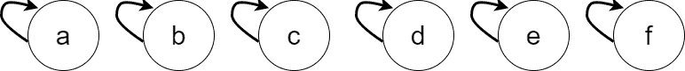
Now, any  returns
  . Let’s unite some of the sets. First, let’s perform
  and
and  . The resulting forest is:
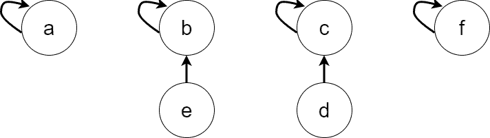
Now, and  belong to the same set, and is the representative of that set, so
  . Similarly,
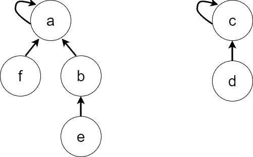
  . Second, let’s perform
  , and then . We get the forest:
4. Pseudocode for the Naive Versions of the Operations
The Naive versions of the operations implement the ideas discussed so far. simply creates a tree with a single node for the element , and the parent link of the node points to itself. For clarity, we’d need an auxiliary operation  , which creates the initial node of a tree:
algorithm CREATE_NODE(a):
    // INPUT
    //    a = an element
    // OUTPUT
    //    A = a node containing a as the value and pointing to itself

    A <- new node
    A.parent <- A
    A.value <- a

    return A
The pseudocode for is as simple as:
algorithm MAKE_SET(a):
    // INPUT
    //    a = an element
    // OUTPUT
    //    The tree containing only the root node with a as its value

    return CreateNode(a)
returns the node with the representative element of the set to which the element belongs. To achieve that, we start from the node containing the element and follow the parent links until we find a node  for which
  :
:
algorithm FIND_SET(A):
    // INPUT
    //    A = the node containing the element a
    // OUTPUT
    //    R = the node which is the root of A's tree

    while A != A.parent:
        A <- A.parent

    return A
appends the root of the  tree to the root of the
  tree:
tree:
algorithm UNION(A, B):
    // INPUT
    //    A = the node containing the element a
    //    B = the node containing the element b
    // OUTPUT
    //    The trees containing A and B are united and the root node of the resulting tree is returned

    if A != B:
        B.parent <- A

    return A
5. The Complexity of the Operations
is a constant operation as it creates a tree node and puts the set element into the created root node.
is a linear operation. Indeed, its complexity depends on the height of the tree to which belongs, and we can come up with a sequence of operations which build a long linear tree. Thus, the naive is an  operation, where is the size of the universe .
is also an operation as it relies on to perform its duty, and besides that it performs  work by reassigning the parent link of the tree.
6. Optimization Strategies
As we see, the bottleneck operation holding DSU back from being a constant time data structure is . Thus, let’s see what optimizations we can perform to make the operation faster.
6.1. Path Compression Heuristics
The first idea is to shorten the tree height during the operation. To do that, we change the parents of all the nodes on the path from node to the root node. How? We make all the parents point directly to the root node. The action has the effect of converting a deep tree into a flat tree. Let’s see an example:
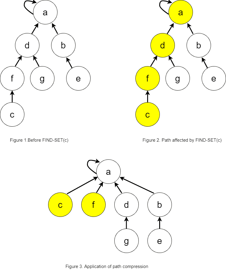
In ‘Figure 1’, we can see the tree prior to performing  operation. ‘Figure 2’ marks the path affected by . Finally, ‘Figure 3’ shows the effect of the path compression heuristics and the marked nodes are the ones which paths have been shortened.
The pseudocode of takes the form:
algorithm FIND_SET(A):
    // INPUT
    //    A = the node containing the element a
    // OUTPUT
    //    R = the node which is the root of A's tree

    if A != A.parent:
        A.parent <- FIND_SET(A.parent)

    return A
Of course, we could implement iteratively, but the recursive version is shorter and more readable.
6.2. Union by Rank Heuristics
The second optimization occurs during the operation. While in the naive implementation of we simply hang the tree on the root of the tree, now we’ll be more selective and won’t allow tree heights to grow fast.
To have a criterion for deciding how to unite two trees, we define the notion of the tree rank. We may define the rank of a tree to be the size of the tree (the number of nodes), though some references define the rank to be the upper bound of the tree’s height. Regardless of the rank selection approach, we hang the tree with the smaller rank to the root of the tree with the bigger rank. When the ranks are equal, we can select the tree to be hung arbitrarily. Also, let’s pay attention to the fact that path compression doesn’t change tree ranks regardless of the rank selection approach.
For our discussion, let’s choose the tree-size approach for the rank. The example below demonstrates the union by rank heuristics:
The rank of the left tree in ‘Figure 4’ is three, while the rank of the right tree is two. Thus, we hang the right tree on the root of the left tree. We can see the result of the operation in ‘Figure 5’.
The pseudocode of with union by rank takes the form:
algorithm UNION(A, B):
    // INPUT
    //    A = the node containing the element a
    //    B = the node containing the element b
    // OUTPUT
    //    The trees containing A and B are united, and the root node of the resulting tree is returned

    A <- FIND_SET(A)
    B <- FIND_SET(B)

    if A = B:
        return A

    newRank <- A.rank + B.rank

    if A.rank >= B.rank:
        B.parent <- A
        A.rank <- newRank
        return A
    else:
        A.parent <- B
        B.rank <- newRank
        return B
Though the union by rank heuristics is performed in the operation, it speeds up . is optimized indirectly as it depends on .
7. The Complexity of the Operations with the Optimizations
The modified operations with the optimizations applied are estimated using the amortized analysis. We’ll only provide the results of optimizations without digging into the details of complexity analysis as it’s vast and complex.
It turns out that each optimization separately speeds up the operations. But when the two optimizations are applied together, they make the DSU operations run in  time, where
  is the inverse Ackermann function. is a very slowly growing function and for any possible practical value of ,
  . Thus, practically all the DSU operations run in constant time on average.
A detailed analysis of the complexity can be found in chapter 21.4 of the book “Introduction to Algorithms, third edition” by Thomas H. Cormen et al.
8. Application in Graph Problems
There are some practical applications of DSU in graph problems. Let’s denote an undirected graph by  , the graph vertices by
  , and the graph edges by
  . We’ll assume the graph has
  vertices and
  edges.
8.1. Finding the Connected Components of an Undirected Graph
The problem of finding the connected components appear in various applications. For example, imagine a black-and-white picture where we want to count the number of black regions. The pixels of the image can be treated as vertices of the graph, and two adjacent pixels are connected with the edge if they have the same color. We can solve the problem using DSU.
The algorithm of finding the connected components is simple: initialize DSU with  . Then, iterate over the edges of the graph and unite the sets of the two vertices of each edge. In the end, each set represents a connected component:
algorithm FindingConnectedComponentsUsingDSU(G):
    // INPUT
    //    G = a graph
    // OUTPUT
    //    The connected components in the form of DSU sets

    for v in G.V:
        MAKE-SET(v)

    for e in G.E:
        UNION(e.v1, e.v2)
Additionally, we might need to perform a linear scan over the vertices of the graph to see which connected component each vertex belongs to. The algorithm complexity is  .
.
The problem of finding the connected components can also be solved using DFS or BFS algorithms which have the same complexity (though they are easier to implement). DSU wins over DFS or BFS for solving the problem when there’s an additional condition to preserve the connected components’ information while adding new edges to the graph.
8.2. Usage of DSU in Kruskal’s Algorithm
Another popular usage of DSU is in the Kruskal’s algorithm for finding the minimum spanning tree of an undirected graph. The straightforward implementation of Kruskal’s algorithm runs in  time. DSU improves the asymptotic to be
  .
.
In Kruskal’s algorithm, we first sort the edges by their weights in increasing order. Then, we iterate over the sorted edges in increasing order of weights, and we unite the sets of each edge’s vertices if they are in different sets (connected components). In a connected undirected graph, there can be a maximum of  union operations, after which we get the minimum spanning tree:
algorithm KruskalsAlgorithm(G):
    // INPUT
    //    G = a graph
    // OUTPUT
    //    MST = the minimum spanning tree as a set of edges

    Sort G.E in ascending order of weights

    for v in G.V:
        MAKE-SET(v)

    MST <- an empty set

    for e in G.E:
        V1 <- FIND-SET(e.v1)
        V2 <- FIND-SET(e.v2)

        if V1 != V2:
            Add e to MST
            UNION(e.v1, e.v2)

    return MST
9. Conclusion
In this article, we introduced the DSU data structure, defined its operations, and described the best representation of DSU as a forest of trees. Then we demonstrated ways to optimize the operations to create a near-constant time data structure. Additionally, we showed some of the applications of DSU in graph problems.