The Direct Linear Transform | Baeldung on Computer Science

1. Introduction

This tutorial introduces the Direct Linear Transform (DLT), a general approach designed to solve systems of equations of the type:

$\lambda\mathbf{x}_k=\mathbf{A} \mathbf{y}_k \text { for } k=1, \ldots, N$

This type of equation frequently appears in projective geometry. One very important example is the relation between 3D points in a scene and their projection onto the image plane of a camera. That is why we’re going to use this setting to motivate the usage of DLT.

2. The Camera Model

The most commonly used mathematical model of a camera is the so-called pinhole camera model. Since the idea of a camera is to map between real-world objects and 2d representations the camera model consists of several coordinate systems:

2.1. Global Coordinates

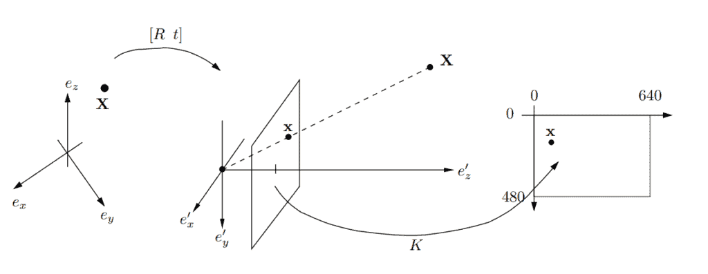
To encode camera position and movement we use the reference coordinate system $\mathbf{\{e_x, e_y, e_z\}}$ (left part of the diagram). In this system, the camera can undergo translation and rotation. The translation is represented as a vector $t \in R$ and the rotation is represented as a $3\times3$ rotation matrix $R$ .

Usually, all the scene point coordinates are also specified in the global coordinate system and $R$ and $t$ are used to relate them to the camera coordinate system as so:

$\left(\begin{array}{l}X_1^{\prime} \\ X_2^{\prime} \\ X_3^{\prime}\end{array}\right)=R\left(\begin{array}{c}X_1 \\ X_2 \\ X_3\end{array}\right)+t .$

Which can be neatly represented in matrix form if we add 1 as an extra dimension.

$\left(\begin{array}{l}X_1^{\prime} \\ X_2^{\prime} \\ X_3^{\prime}\end{array}\right)=\left[\begin{array}{ll}R & t\end{array}\right]\left(\begin{array}{c}X_1 \\ X_2 \\ X_3 \\ 1\end{array}\right)$

2.2. Camera Coordinates

The camera coordinate system $\mathbf{\{e^\prime_x, e^\prime_y, e^\prime_z\}}$ (in the middle of the diagram) has an origin $\mathbf{C = (0,0,0)}$ which represents the camera center, or pinhole. To generate a projection $x = (x_1, x_2, 1)$ of a scene point $X = (X\prime_1, X\prime_2,X\prime_3)$ we form the line between $X$ and $C$ and intersect it with the plane $Z = 1$ .

This plane is also called the image plane and the line intersecting it is the viewing ray. One might note that unlike a physical camera the projection plane is in front of the pinhole. This is done for convenience and has the effect that the image will not appear upside down as in the real model.

2.3. Inner Parameters

In the pinhole camera model, the image plane lies in $\mathbb{R}^3$ , meaning that the projections are given in the length of real-world units. But when we are talking about images, we use pixels in a specified dimension. In our example diagram, we ‘re using $640 \times 480$ pixels. To convert it we use a mapping (right side of the diagram) from the image plane embedded in $\mathbb{R}^3$ to the real image.

This pixel mapping is represented by an invertible triangular $\mathbf{3\times3}$ matrix $\mathbf{K}$ which contains the inner parameters of the camera, that is, focal length, principal point, aspect ratio, and axis skew.

2.4. Full Representation

And finally, we can relate all three parts of the camera model into one equation:

$\lambda\left(\begin{array}{l}x_1 \\ x_2 \\ 1\end{array}\right)=K\left [\begin{array}{ll}R & t\end{array}\right]\left(\begin{array}{c}X_1 \\ X_2 \\ X_3 \\ 1\end{array}\right)$

or more succinctly:

$\lambda x = PX$

where P is called the camera matrix.

The above equation now looks like the exact type that DLT can help us find the matrix P if we wanted to.

3. Camera Calibration

But why do we need to solve it in the first place? Most of the time we’re interested in finding the $K$ part of the camera matrix $P$ . Because if $K$ is known we can see that the camera is calibrated. And with a calibrated camera we can do things like lens distortion correction, measuring an object from a photo, or even estimating 3d coordinates from camera motion.

To do that we’ll first need at least 6 data points measured by hand, we can then compute the camera matrix P using the DLT method and finally factorize $P$ into $K\left [\begin{array}{ll}R & t\end{array}\right]}$ using RQ-factorization.

4. Method

The first step of the DLT method formulates a homogeneous linear system of equations and solves it by finding an approximate null space. To do that we first express P in terms of row vectors:

$P = \begin{bmatrix} p_1^T \\p_2^T\\p_3^T\end{bmatrix}$

Then we can write the camera equation as:

$\mathbf{X}_i^T p_1-\lambda_i x_i=0$

$\mathbf{X}_i^T p_2-\lambda_i y_i=0$

$\mathbf{X}_i^T p_3-\lambda_i=0$

which in turn can be put into matrix form as such:

$\left[\begin{array}{cccc}\mathbf{X}_i^T & 0 & 0 & -x_i \\ 0 & \mathbf{X}_i^T & 0 & -y_i \\ 0 & 0 & \mathbf{X}_i^T & -1\end{array}\right]\left(\begin{array}{l}p_1 \\ p_2 \\ p_3 \\ \lambda_i\end{array}\right)=\left(\begin{array}{l}0 \\ 0 \\ 0\end{array}\right)$

Note that since $X_i$ is a $4\times 1$ vector each $0$ actually represents a $1\times 4$ block of zeros, meaning we are multiplying a $3 \times 13$ matrix multiplied with a $13\times 1$ vector.

If we stack all the projection equations of all the measured data points in one matrix, we get a system of the form:

$\begin{bmatrix} \mathbf{X}_1^T & 0 & 0 & -x_1 & 0 & 0 & \cdots\\ 0 & \mathbf{X}_1^T & 0 & -y_1 & 0 & 0 & \cdots\\ 0 & 0 & \mathbf{X}_1^T & -1& 0 & 0 & \cdots\\ \mathbf{X}_2^T & 0 & 0 & 0 & -x_2 & 0 & \cdots\\ 0 & \mathbf{X}_2^T & 0 & 0 & -y_2 & 0 & \cdots\\ 0 & 0 & \mathbf{X}_2^T & 0& -1 & 0 & \cdots\\ \mathbf{X}_3^T & 0 & 0 & 0 & 0 & -x_3 & \cdots\\ 0 & \mathbf{X}_3^T & 0 & 0 & 0 & -y_3 & \cdots\\ 0 & 0 & \mathbf{X}_3^T & 0 & 0 & -1 & \cdots\\ \vdots & \vdots & \vdots & \vdots & \vdots & \vdots & \ddots \end{bmatrix} \left(\begin{array}{l}p_1 \\ p_2 \\ p_3 \\ \lambda_1\\\lambda_2\\\lambda_3\\\vdots\end{array}\right) = \left(\begin{array}{l}0 \\ 0 \\ 0 \\ 0 \\0 \\ 0 \\0 \\ 0 \\0 \\ \vdots\end{array}\right)$

$\bigbreak$

$Mv=0$

After rearranging the equations, we just need to find a non-zero vector in the null space of $M$ to solve the system. In most cases, however, there will not be an exact solution due to noise while measuring. Therefore, it is more convenient to search for a solution that minimizes the total error essentially solving a least square problem instead.

One way of solving it is to use Singular Value Decomposition (or SVD). After decomposing the big matrix $M$ we can take the right singular vector corresponding to the smallest singular value and we have found the camera matrix $P$ . We can then factorize $P$ into $K\left [\begin{array}{ll}R & t\end{array}\right]}$ using the QR-factorization method, as mentioned before.

5. Conclusion

In this article, we looked into the pinhole camera model and motivated the usage of the Discrete Linear transformation (DLT) by trying to find the intrinsic parameters of a given camera model. Using this setting as an example we looked into the methodology behind the approach and how it works.

Full Archive

About Baeldung

Core Concepts

Operating Systems

Artificial Intelligence

Graph Theory

Latex