Correcting Fisheye Images | Baeldung on Computer Science

1. Introduction

Fisheye lenses have become a staple in creative photography alongside other tilt-shift, telephoto zoom, and wide-angle lenses. This lens type applies a different distortion (or projection) mapping than a regular “pinhole” camera.

In this tutorial, we’ll demonstrate how to undo this distortion and extract a “straight” image from a fisheye photograph.

2. Understanding Camera Parameters

Essentially, we are interested in estimating the $P$ transformation involved in projecting a 3D point in space $X$ onto a projected 2D coordinate $x$ as follows:

$x = PX$

This $P$ transform can further be divided into 5 intrinsic and 6 extrinsic parameters.

$x = K R [I_3|-X_0] X$

2.1. Extrinsic Parameters

Extrinsic parameters in computer vision deal with the camera’s position (physical location in $X$ , $Y$ , and $Z$ but also the pose of the camera) relative to the world reference or origin.

In $P$ , these are referenced as three rotations $R$ and three translations $[I_3|-X_0]$ along the width, height, and depth dimensions.

2.2. Intrinsic Parameters

Intrinsic parameters in computer vision deal with the camera’s ability to map out points in the real world with respect to a 2D “sensor” or “film”. We are interested in these parameters for applying and correcting lens distortions.

Literature dealing with intrinsic camera parameters in computer vision often references a 3 x 3 camera matrix, which we’ll denote as $\mathbf{K}$ . In order to understand better these fundamental optical matrices and how to multiply them, we can look at this interactive website.

This is what this K matrix can look like:

$K =\begin{pmatrix}f_x & s & x_0 \\0 & f_y & y_0\\0 & 0 & 1 \end{pmatrix}$

The elements in the matrix can be decomposed as follows:

$F_x$ and $F_y$ denote the focal lengths in $y$ and $x$ respectively.
$s$ denotes a shear transformation
$x_0$ and $y_0$ denote translations along $x$ and $y$ respectively

This K matrix corresponds to this camera matrix detailed in OpenCV’s literature.

2.3. Total Parameters

After some simplifications, we have the resulting total transform matrix:

$\begin{pmatrix}x\\ y \\1 \end{pmatrix} =\begin{pmatrix}f_x & s & x_0 \\0 & f_y & y_0\\0 & 0 & 1 \end{pmatrix}\begin{pmatrix}r_1_1 & r_1_2 & t_1 \\ r_2_1 & r_2_2 & t_2\\r_3_1 & r_3_2 & t_3 \end{pmatrix}\begin{pmatrix}X\\ Y \\1 \end{pmatrix}$

or alternatively:

$\begin{pmatrix}x\\ y \\1 \end{pmatrix} = K [r_1,r_2,t] \begin{pmatrix}X\\ Y \\1 \end{pmatrix}$

We can represent the target coordinated only with $X$ and $Y$ because we assume that our calibration target is flat. This is usually a printed checkerboard.

3. Types of Fisheye Lenses

Fisheye lenses are not all created equal. In order to know how to correct the distortion on a fisheye lens, it could be helpful to know what kind of fisheye we’re dealing with to better approximate its focal lengths “ $F(x | y)$ “. Fisheye lenses can be rectilinear, stereographic, equidistant, equisolid angle, or orthographic. Here is a list of different types and their respective focal functions.

The $\theta$ angle referenced is the angle from the lens’s optical axis.

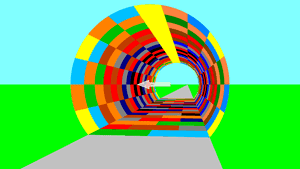
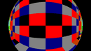
We will use the following image to present the different alternatives. The camera faces the left inside the colorful cylinder, as indicated by the arrow.

3.1. Rectilinear

This lens works like a pinhole camera, which means that straight lines will remain straight in the resulting image. $θ$ has to be smaller than 90°. The aperture angle is gaged symmetrically to the optical axis and has to be smaller than 180°:

Large aperture angles are challenging to design and lead to high prices.

3.2. Stereographic

This fisheye lens type maintains angles. This mapping doesn’t compress objects in the margin of the photograph as much as others:

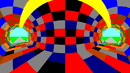
Below are some examples of this fisheye lens type:

Samyang f = 8 mm f/2.8
Samyang f = 12 mm f/2.8

3.3. Equidistant

In contrast to the previous type, the equidistant fisheye lens maintains angular distances. This can be interesting for angle measurement applications. PanoTools uses this type of mapping:

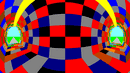
Below are some examples of this fisheye lens type:

Canon FD f = 7.5 mm f/5.6
Coastal Optical f = 7.45 mm f/5.6
Nikkor f = 6 mm f/2.8
Nikkor f = 7.5 mm f/5.6
Nikkor f = 8 mm f/2.8
Nikkor f = 8 mm f/8.0
Peleng f = 8 mm f/3.5
Rokkor f = 7.5 mm f/4.0
Sigma f = 8 mm f/3.5
Samyang f = 7.5 mm f/3.5

3.4. Equisolid Angle

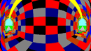
Alternatively, the equisolid angle fisheye lens maintains surface relations. The resulting image looks like a reflective surface of a sphere. This is a common type of fisheye lens. In comparison to the stereographic lens, this one does compress the margins.

Below are some examples of this fisheye lens type:

Canon EF f = 15 mm f/2.8 (1988)
Minolta f = 16 mm f/2.8 (1971)
Nikkor f = 10.5 mm f/2.8
Nikkor f = 16 mm f/2.8 (1995)
Sigma f = 4.5 mm f/2.8
Sigma f = 8 mm f/4.0
Sigma f = 15 mm f/2.8 (1990)
Zuiko f = 8 mm f/2.8

3.5. Orthographic

Orthographic lenses maintain planar illuminance. The center image is less compressed, however, the margins are very much distorted:

Below are some examples of this fisheye lens type:

Nikkor f = 10 mm f/5.6 OP
Yasuhara Madoka180 f = 7.3 mm f/4

Once we know the type of sensor (APS-C, 35mm, etc.) and the focal length of our lens, we can simply calculate F(x,y) depending on our lens type or pick a value from the table in this list.

4. Example

Finally, we can quickly test this new knowledge on our browse using FisheyeGl (a library for correcting fisheye, or barrel distortion, on browser images that require JavaScript with WebGL).

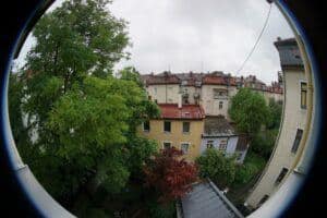
We’re going to use this APS-C, 75mm fisheye photograph for our experiment, which employs a very radical fisheye look:

Firstly, we can load the photograph onto the application:

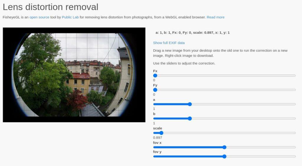
We can see the different settings available, and we can recognize some of them, however, two new ones appear. These parameters a and b are the radial and tangential distortion coefficients, respectively.

We can then apply the following settings:

$F_x$ = 0.26
$F_y$ = 0.26
$Scale$ = 0.7
$a$ and $b$ can remain at their default “1” value

Finally, we can extract the following photograph:

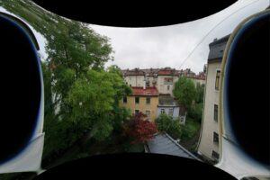
We can see how the picture is re-distorted to achieve straighter lines on the edges of the resulting image. We can also note that the artifacts at the edges of the screen are very much warped. We can also note that the dimensions of the resulting image are more significant than the original. This is why we set the scale to 0.7.

By manually adjusting the radial and tangential distortion parameters, we could perhaps achieve a finer result, however, modeling these as linear across the entire image, this model limits us.

5. Distortion & Camera Calibration

Alternatively, suppose we are trying to work with a specific camera, and we need to be very careful with approximating its resulting undistorted image. In that case, it is best to use a target. Even some “pinhole” cameras may require this treatment for downstream tasks as many lenses can introduce distortion in the image that the intrinsic parameters and linear distortion cannot model. Target-less calibration can only be precise because the model we’re using is limited.

Therefore, we can have a much finer model by approximating radial and tangential distortion coefficients through calibration. A standard practice in computer vision is to observe a target with known structure and dimensions and use a method to obtain the position of the different calibration points in the image. This is called photogrammetric calibration.

Targets for color cameras look like checkerboards like this one:

5.1. Zhang’s Method

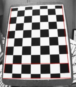
This particular method for camera calibration was introduced in a Flexible New Technique For Camera Calibration in 1999.

5.2. Linear Parameters

We can say that each point in the checkerboard will generate the following (previous equation):

We can use this equation to define a homography matrix $H$ as follows:

$H = [h_1, h_2, h_3] =\begin{pmatrix}f_x & s & x_0 \\0 & f_y & y_0\\0 & 0 & 1 \end{pmatrix}\begin{pmatrix}r_1_1 & r_1_2 & t_1 \\ r_2_1 & r_2_2 & t_2\\r_3_1 & r_3_2 & t_3 \end{pmatrix}$

We can now estimate a 3×3 homography matrix instead of a 3×4 projection matrix. To solve for $H$ , we need to observe at least 4 points as $H$ has 8 degrees of freedom (DoF), and each point consists of a pair of $x,y$ coordinates.

To compute $K$ from $H$ , this method relies on four steps:

Exploiting constraints about $K, r_1, r_2$
Defining a matrix $B = K^{-T} K^{-1}$
Computing $B$ by solving a homogenous linear system
Decomposing $B$ to find $K$

5.3. Non-Linear Parameters

The most common approach to estimate non-linear (distortion) parameters of a lens is to model them using the following equations:

$x^a = x(1+q_1 r^2 + q_2 r^4)$ and $y^a = y(1+q_1 r^2 + q_2 r^4)$

In this case, $r$ represents the distance between the pixel in the image and the principal point.

Also $[x,y]^T$ is the point as projected by an ideal pinhole camera. $q_1$ and $q_2$ are additional non-linear parameters.

Lens distortion can finally be approximated by minimizing the following error function:

$\Sigma_n\Sigma_i || x_{ni}-\^{x}(K,q,R_n,t_n,X_{ni})||^2$

6. OpenCV Implementation

One of the best computer vision libraries out there is OpenCV.

Using tutorials from libraries like OpenCV, we can automatically detect the corners on the checkerboard and extract an intrinsic parameter camera matrix and display them on the image:

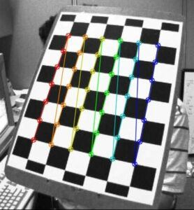
By taking multiple pictures, each mapping out more calibration points in our camera sensor, we can more accurately estimate the camera’s intrinsic parameters along with the distortions in the image.

Additional information can be found in this tutorial.

If we were using a thermal camera, there are other calibration target types available that we could leverage. However, the procedure would be the same.

7. Conclusion

In this article, we reviewed different methods for programmatically correcting fisheye images.

Full Archive

About Baeldung

Core Concepts

Operating Systems

Artificial Intelligence

Graph Theory

Latex

1. Introduction

2. Understanding Camera Parameters

2.1. Extrinsic Parameters

2.2. Intrinsic Parameters

2.3. Total Parameters

3. Types of Fisheye Lenses

3.1. Rectilinear

3.2. Stereographic

3.3. Equidistant

3.4. Equisolid Angle

3.5. Orthographic

4. Example

5. Distortion & Camera Calibration

5.1. Zhang’s Method

5.2. Linear Parameters

5.3. Non-Linear Parameters

6. OpenCV Implementation

7. Conclusion