Negative Weights Using Dijkstra’s Algorithm

1. Overview

In this tutorial, we’ll discuss the problems that occur when using Dijkstra’s algorithm on a graph with negative weights.

First, we’ll recall the idea behind Dijkstra’s algorithm and how it works.

Then we’ll present a couple of issues with Dijkstra’s algorithm on a graph that has negative weights.

2. Recall Dijkstra’s Algorithm

2.1. Main Idea

Suppose we have a graph, , that contains nodes numbered from to . In addition, we have edges that connect these nodes. Each of these edges has a weight associated with it, representing the cost to use this edge. Dijkstra’s algorithm will give us the shortest path from a specific source node to every other node in the given graph.

Recall that the shortest path between two nodes, and , is the path that has the minimum cost among all possible paths between and .

2.2. Implementation

Let’s take a look at the implementation:

algorithm Dijkstra(V, G):
    // INPUT
    //    V = Number of nodes in the graph
    //    G = The graph stored as an adjacency list
    // OUTPUT
    //    Returns the cost of the shortest path 
    //    from a source node to every other node in G
    
    cost <- [infinity for node in G]
    priority_queue <- an empty priority queue
    // the queue will be ordered based on the cost array
    
    priority_queue.add(source_node)
    cost[source_node] <- 0
    
    while priority_queue is not empty:
        current <- priority_queue.front()
        priority_queue.pop()
    
        for neighbor in neighbors(current):
            edge_cost <- weight(current, neighbor)
            if cost[neighbor] > cost[current] + edge_cost:
                priority_queue.add(neighbor)
                cost[neighbor] <- cost[current] + edge_cost
    
    return cost

Initially, we declare an array called , which stores the shortest path between the source node and every other node in the given graph. In addition, we declare a priority queue that stores the explored nodes and keeps them sorted in ascending order according to their cost value.

Next we add the source node to the priority queue and make the cost to reach the source node equal to , since the shortest path from a node to itself is equal to zero. Then we perform multiple steps as long as the queue isn’t yet empty. In each step, we take the node with the minimum cost from the queue. Since the queue is sorted based on each node’s cost, the one with the minimum cost will be located at the front of the priority queue.

After that, we check whether it has a better cost for each neighbor of the current node than the newly discovered one. The new cost equals the cost of reaching the current node, plus the weight of the edge that connects the current node with its neighbor. If the new cost is lower, we found a new path from the source node to this neighbor by reaching it through the current node. In this case, we’ll update the neighbor’s cost and add it to the priority queue.

Finally, we return the array, which stores the shortest path from the source node to every other node in the given graph.

2.3. Proof of Concept

The proof of correctness for Dijkstra’s algorithm is based on the greedy idea that if there was a shorter path than any sub-path, then the shorter path should replace that sub-path to make the whole path shorter. Let’s illustrate this idea better.

In each step of Dijkstra’s algorithm, we know the shortest paths so far (each node inside the queue represents a unique path from the source to this node). However, this means that we could find better paths in later steps once we explore more nodes. Therefore, we can’t be sure of whether the current discovered paths are the shortest ones.

Nevertheless, we can be sure of exactly one path, which is the one with the lowest cost inside the queue. The reason is that the other paths have a higher cost. So to reach the end node of the path with the lowest cost, we’ll need to use a few extra edges, resulting in a higher cost. Thus, we always pick the path with the lowest cost and explore the next nodes to this path.

Keep in mind that our assumption is based on the idea that all edges have a non-negative weight. Otherwise, we can’t be certain about choosing the path with the lowest cost. The reason is that choosing a different path with a higher cost might give us a lower total cost when we explore some negative-cost edges from that path.

In the next sections, we’ll describe two cases that fail with Dijkstra’s algorithm because some edges have negative costs.

3. Infinite Cycles

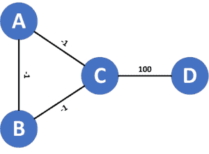
Let’s take a look at the following graph:

Let the source node be . When we run Dijkstra’s algorithm from , we’ll add and to the priority queue, both with a cost equal to .

Next, we’ll pop node because it has the minimum cost among all nodes in the priority queue, and we’ll add nodes and , both with a cost equal to . In the next step, we pop node and add nodes and , both with the cost equal to . Then we go back to node .

The same scenarios will happen repeatedly; as we can see, we’ll be stuck in an infinite cycle because in each iteration, we’ll get a smaller cost, and we’ll never reach node using Dijkstra’s algorithm.

In conclusion, Dijkstra’s algorithm never ends if the graph contains at least one negative cycle. By a negative cycle, we mean a cycle that has a negative total weight for its edges.

4. Wrong Path

Let’s take a look at the following graph:

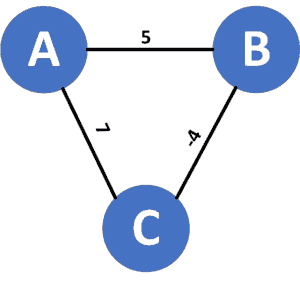
Let be the source node. When we run Dijkstra’s algorithm from , we’ll add and to the priority queue with costs equal to and , respectively.

Next, we’ll pop node , since it has the minimum cost among all nodes in the priority queue, and add node with a cost equal to . Finally, we pop node , and Dijkstra’s algorithm will stop here.

The array will look like this, , representing the cost of the shortest path to reach nodes , , and , respectively. However, we can reach node with a cost equal to through the path .

What happened is that we didn’t go through the because we reached node with a smaller cost, and we ignore all paths that pass through using this greedy approach.

To conclude this case, Dijkstra’s algorithm can reach an end if the graph contains negative edges, but no negative cycles; however, it might give wrong results.

5. Conclusion

In this article, we recalled Dijkstra’s algorithm and provided two scenarios in which it fails on negative edges.