Detecting Cycles in a Directed Graph

1. Introduction

Directed graphs are usually used in real-life applications to represent a set of dependencies. For example, a course pre-requisite in a class schedule can be represented using directed graphs.

And cycles in this kind of graph will mean deadlock — in other words, it means that to do the first task, we wait for the second task, and to do the second task, we wait for the first. So, detecting cycles is extremely important to avoid this situation in any application.

2. Problem Explanation

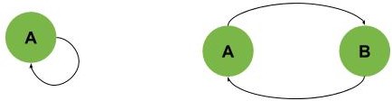
In a directed graph, we’d like to find cycles. These cycles can be as simple as one vertex connected to itself or two vertices connected as shown:

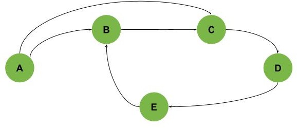
Or, we can have a bigger cycle like the one shown in the next example, where the cycle is B-C-D-E:

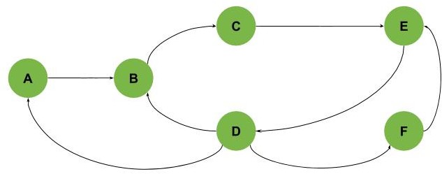
Also, we can get graphs with multiple cycles intersecting with each other as shown (we have three cycles: A-B-C-E-D, B-C-E-D, and E-D-F):

We should also notice that in all previous examples, we can find all cycles if we traverse the graphs starting from any node. However, this isn’t true in all graphs.

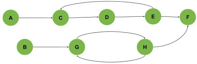
In some graphs, we need to start visiting the graph from different points to find all cycles as in the graph, as shown in the following example (Cycles are C-D-E and G-H):

3. Algorithm Idea

Finding cycles in a simple graph as in the first two examples in our article is simple. We can traverse all the vertices and check if any of them is connected to itself or connected to another vertex that is connected to it. But, of course, this isn’t going to work in more complex scenarios.

So, one famous method to find cycles is using Depth-First-Search (DFS). By traversing a graph using DFS, we get something called DFS Trees. The DFS Tree is mainly a reordering of graph vertices and edges. And, after building the DFS trees, we have the edges classified as tree edges, forward edges, back edges, and cross edges.

Let’s see an example based on our second graph:

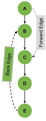
We can notice that the edge E-B is marked as a back edge in the previous example. A back edge is an edge that is connecting one of the vertices to one of its parents in the DFS Tree.

In the previous example, we also have the edge A-C marked as a forward edge. A forward edge is an edge connecting a parent to one of the non-direct children in the DFS tree.

Notice that we also have the normal edges in solid lines in our graph. These solid line edges are the tree edges. The Tree edges are defined as the edges that are the main edges visited to make the DFS tree. 

Let’s see another example where we have multiple back edges:

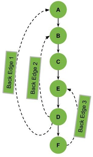
Notice that with each back edge, we can identify cycles in our graph. So, if we remove the back edges in our graph, we can have a DAG (Directed Acyclic Graph).

Now, let’s see one final example to illustrate another issue we might face:

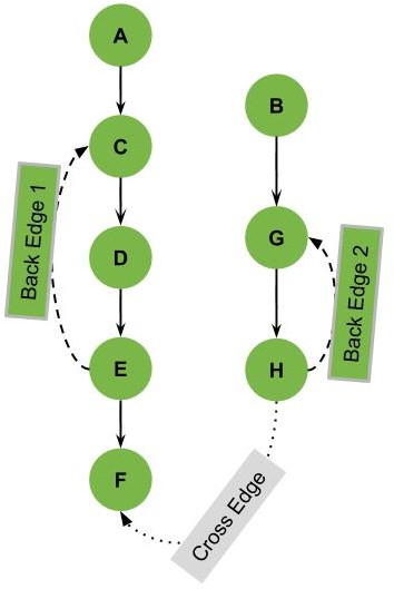
In this last example, we can see an edge marked as a cross edge.

To understand this part, we need to think of the DFS over the given graph. If we start the DFS on this graph starting from vertex A, we’ll visit the vertices A, C, D, E, and F.

Still, we’ll not see the vertices B, G, and H. So, in this case, we need to restart the DFS after the first run from a different point that was not visited, such as the vertex B. As a result of these multiple DFS runs, we’ll have multiple DFS Trees.

To conclude the idea in this example, we can have multiple DFS trees for a single graph. And the cross edge is in our example is the edge connecting vertex from one of the DFS trees to another DFS tree in our graph.

A cross edge can also be within the same DFS tree if it doesn’t connect a parent and child (an edge between different branches of the tree).

However, in this tutorial, we’re mainly interested in the back edges of the DFS tree as they’re the indication for cycles in the directed graphs.

4. Flow-Chart

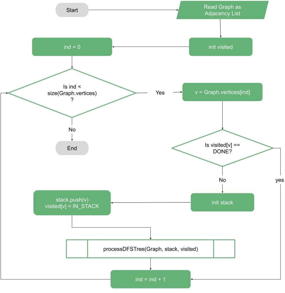
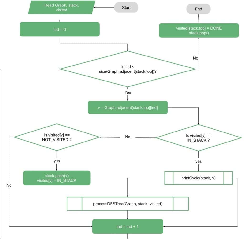
We can illustrate the main idea simply as a DFS problem with some modifications. The first thing is to make sure that we repeat the DFS from each unvisited vertex in the graph, as shown in the following flow-chart:

The second part is the DFS processing itself. In this part, we need to make sure we have access to what is in the stack of the DFS to be able to check for the back edges.

And whenever we find a vertex that is connected to some vertex in the stack, we know we’ve found a cycle (or multiple cycles):

If our goal is to print the first cycle, we can use the illustrated flow-chart to print the cycle using the DFS stack and a temporary stack:

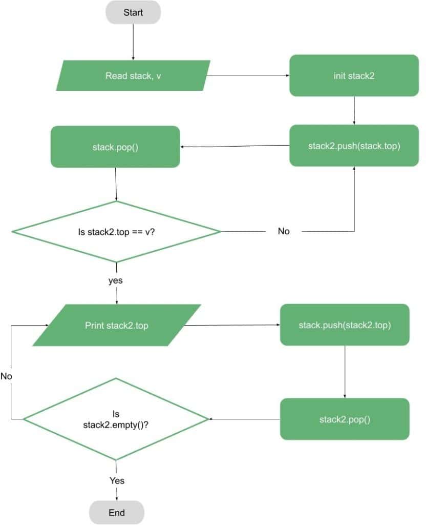
However, if our goal is to convert the graph to an acyclic graph, then we should not print the cycles (as printing all cycles is an NP-Hard problem).

Instead, we should mark all the back edges found in our graph and remove them.

5. Pseudocode

Our next part of this tutorial is a simple pseudocode for detecting cycles in a directed graph.

In this algorithm, the input is a directed graph. For simplicity, we can assume that it’s using an adjacency list.

The first function is an iterative function that reads the graph and creates a list of flags for the graph vertices (called visited in this pseudocode) that are initially marked as NOT_VISITED.

Then, the function iterates over all the vertices and calls the function processDFSTree when it finds a new NOT_VISITED vertex:

algorithm findCycles(Graph):
    // INPUT
    //   Graph = a graph
    // OUTPUT
    //   Print all cycles in the graph

    visited <- array of NOT_VISITED for each vertex in Graph
    for each vertex v in Graph.vertices:
        if visited[v] == NOT_VISITED:
            stack <- empty stack
            stack.push(v)
            visited[v] <- IN_STACK
            detectedCycles <- empty list
            processDFSTree(Graph, stack, visited, detectedCycles)

The processDFSTree function is a recursive function that takes three inputs: the graph, the visited list, and a stack. After that, the function is mainly doing DFS, but it also marks the found vertices as IN_STACK when they’re first found.

And after processing the vertex, we mark it as DONE. In case we find a vertex that is IN_STACK, we’ve found a back edge, which indicates that we’ve found a cycle (or cycles).

So, we can print the cycle or mark the back edge:

algorithm processDFSTree(Graph, Stack, visited, detectedCycles):
    // INPUT
    //   Graph = a graph
    //   Stack = current path
    //   visited = a visited set
    //   detectedCycles = a collection of already processed cycles
    // OUTPUT
    //   Print all cycles in the current DFS Tree

    for each vertex v in Graph.adjacent[Stack.top]:
        if visited[v] == IN_STACK:
            printCycle(Stack, v, detectedCycles)
        else if visited[v] == NOT_VISITED:
            Stack.push(v)
            visited[v] <- IN_STACK
            processDFSTree(Graph, Stack, visited, detectedCycles)

    visited[Stack.top] <- NOT_VISITED
    Stack.pop()

Finally, let’s write the function that prints the cycle:

algorithm printCycle(Stack, v, detectedCycles):
    // INPUT
    //   Stack = current path
    //   v = current node
    //   detectedCycles = a collection of already processed cycles
    // OUTPUT
    //   Print the cycle that lives in the stack starting from vertex v

    cycle <- empty list
    cycle.push(Stack.top)
    Stack.pop()
    while cycle.top != v:
        cycle.push(Stack.top)
        Stack.pop()

    if cycle not in detectedCycles:
        detectedCycles.push(cycle)
        print(cycle)

The printing function mainly needs the stack and the vertex that was found with the back edge. Then, the function pops the elements from the stack and prints them, then pushes them back, using a temporary stack.

6. Complexity

The given algorithm’s time complexity is . This significant performance penalty comes from the fact that we’re trying to find all the cycles to print them. As for the space complexity, we also get due to the fact that we need to store detected cycles to avoid printing them again.

It’s easy to visualize this case in a graph where all the nodes are connected. The cycles would contain all the possible permutations with lengths from 1 to .

However, if we don’t need to find all the cycles and just check if a graph contains any cycles at all, we can simplify the provided Algorithm 2:

algorithm containsCycle(Graph, Stack, visited):
    // INPUT
    //   Graph = a graph
    //   Stack = current path
    //   visited = a visited set
    // OUTPUT
    //   Checks if a given graph contains cycles

    for each vertex v in Graph.adjacent[Stack.top]:
        if visited[v] == IN_STACK:
            return True
        else if visited[v] == NOT_VISITED:
            Stack.push(v)
            detectedCycles <- empty list
            visited[v] <- IN_STACK
            if processDFSTree(Graph, Stack, visited, detectedCycles):
                return True

    visited[Stack.top] <- NOT_VISITED
    Stack.pop()
    return False

The version of the algorithm mainly represented by DFS, and the time complexity would be . We need to allocate space for marking the vertices and the stack so that the space complexity will be in the order of

Please note that Algorithm 1 should have minor changes to work with this version and handle the result. However, they’re trivial and not presented here.

7. Conclusion

In this tutorial, we covered one of the algorithms to detect cycles in directed graphs. At first, we discussed one of the important applications for this algorithm. Then, we explained the idea and showed the general algorithm idea using examples, flow-charts, and pseudocode.

Finally, we showed an average space and time complexity for the algorithm.