

Learn through the super-clean Baeldung Pro experience:
>> Membership and Baeldung Pro.
No ads, dark-mode and 6 months free of IntelliJ Idea Ultimate to start with.
Last updated: March 18, 2024
Learn through the super-clean Baeldung Pro experience:
>> Membership and Baeldung Pro.
No ads, dark-mode and 6 months free of IntelliJ Idea Ultimate to start with.
The problem of choosing a subarray that fulfills some conditions can have many versions. In this tutorial, we’ll discuss finding the subarray with the closest sum to a target number without exceeding it.
We’ll discuss multiple solutions and provide a comparison between them.
The problem gives us an array of size  and a target number
  . We’re asked to find the subarray whose sum is as close to as possible, without exceeding it.
Let’s take the array  as an example:
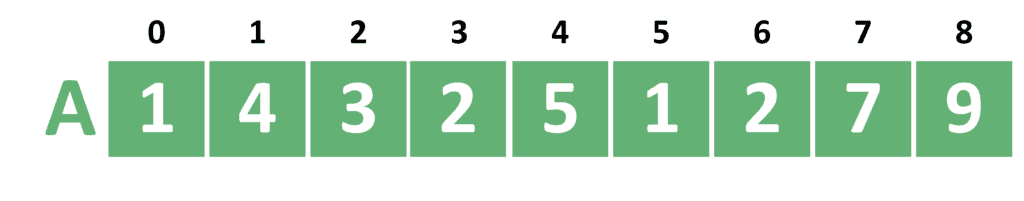
Suppose the target number is  . In this case, we can see that some subarrays, such as
 ![[0..3]](/wp-content/ql-cache/quicklatex.com-177d949d87f23b18e3e4ee672218b293_l3.svg "Rendered by QuickLaTeX.com") and
and ![[5..7]](/wp-content/ql-cache/quicklatex.com-9d34fac73c38db69335886ab89b8ded0_l3.svg "Rendered by QuickLaTeX.com") , have a sum equal to 10. However, the best choice is to choose the subarray
, have a sum equal to 10. However, the best choice is to choose the subarray ![[2..5]](/wp-content/ql-cache/quicklatex.com-f012beea917a328a2fa3398a19605cd7_l3.svg "Rendered by QuickLaTeX.com") because it has a sum of 11. Hence, its sum is just smaller by one from . Also, note that this is the closest we can get to without exceeding it.
because it has a sum of 11. Hence, its sum is just smaller by one from . Also, note that this is the closest we can get to without exceeding it.
We’ll discuss three approaches to solve this problem.
The naive approach checks every possible subarray of the array . Take a look at the implementation of the naive approach:
algorithm NaiveApproach(A, n, k):
    // INPUT
    //    A = The array of elements indexed from 0 to n - 1
    //    n = The size of the array A
    //    k = The target sum
    // OUTPUT
    //    The maximum sum of a subarray of A that does not exceed k

    answer <- 0
    for L <- 0 to n - 1:
        sum <- 0
        R <- L
        while R < n and sum + A[R] <= k:
            sum <- sum + A[R]
            R <- R + 1
        answer <- max(answer, sum)
    return answer
First, we initialize the best answer with zero. Second, we iterate over all possible beginning  of the subarray to take.
From each beginning, we check to see how far this subarray can be extended. Therefore, we keep moving  forward as long as the sum doesn’t exceed . When the current subarray can’t be extended any farther, we compare its sum with the stored answer and keep the maximum between them.
Finally, we return the best answer we managed to find.
It’s important to note that, for each beginning , we’re making the right side of the range start from . Then, we keep moving as far as possible.
Hence, the complexity of the naive approach is  , where is the number of elements inside the array .
The two-pointers approach is an update over the naive approach. Consider the pseudocode implementation of the two-pointers approach:
algorithm TwoPointersApproach(A, n, k):
    // INPUT
    //    A = The array of elements
    //    n = The size of the array A
    //    k = The target sum
    // OUTPUT
    //    The maximum sum of a subarray of A that does not exceed k

    answer <- 0
    sum <- 0
    R <- 0
    for L <- 0 to n - 1:
        if L > 0:
            sum <- sum - A[L - 1]
        while R < n and sum + A[R] <= k:
            sum <- sum + A[R]
            R <- R + 1
        answer <- max(answer, sum)
    return answer
As we can see, the implementation is similar to the naive approach. However, the main difference is that we don’t set the value of to each time.
Instead, we let keep its old value, as well as the sum.
Let’s explain this idea.
Suppose we’re checking a subarray that begins at . Also, let’s assume we managed to find the best ending at . When we move to the next subarray, the one that starts at  , the difference is that the number at index is out of the range. Therefore, we subtract it from the sum.
However, now that the number at index is out of the subarray, we may be able to get new elements to the subarray. Hence, we check to see how far can we push forward, without having the sum exceed .
Although the complexity may sound similar to the naive approach, the complexity of the two-pointers approach is  , where is the number of elements inside the array . The reason is that never goes back. As a result, the inner
  loop gets executed at most times in total.
The problem with the first two approaches is that we assumed there’d be no negative values. Hence, whenever the sum of a subarray exceeds , we always stop and check the answer.
On the other hand, the prefixes approach handles the problem even if the array contains negative values.
Let’s have a quick background of prefix sum; then we can jump into the third approach to solve this problem.
Suppose the problem was to answer some queries that ask for the sum of a certain subarray. In this case, we can calculate the prefix array in advance. Each index inside the prefix array ![prefix[i]](/wp-content/ql-cache/quicklatex.com-814bb8b608f1ff405a6a5ddee5481e06_l3.svg "Rendered by QuickLaTeX.com") holds the sum of the prefix that ends at the index
holds the sum of the prefix that ends at the index  .
.
In other words, holds the sum of the range ![[0..i]](/wp-content/ql-cache/quicklatex.com-c7ff26c3afbff324f5821772ab10896d_l3.svg "Rendered by QuickLaTeX.com") . For simplicity, we’ll shift the
. For simplicity, we’ll shift the  array by one. Hence,
 ![prefix[i+1]](/wp-content/ql-cache/quicklatex.com-038d67e1c28591c99ca9817e63f1faef_l3.svg "Rendered by QuickLaTeX.com") will hold the sum for the subarray . Also,
will hold the sum for the subarray . Also, ![prefix[0]](/wp-content/ql-cache/quicklatex.com-c5728fa48c7565d69a2bb711ed35cf94_l3.svg "Rendered by QuickLaTeX.com") will equal 0 indicating the empty prefix.
will equal 0 indicating the empty prefix.
To calculate the sum of a certain range ![[L, R]](/wp-content/ql-cache/quicklatex.com-aeea634230c22e2940acb7070696d9ef_l3.svg "Rendered by QuickLaTeX.com") inside the array, we can split this range into two ranges.
inside the array, we can split this range into two ranges.
The first range is ![[0, R]](/wp-content/ql-cache/quicklatex.com-3ab249afe85c8030c90819ad54e3ba6f_l3.svg "Rendered by QuickLaTeX.com") , which contains the needed rage with some extra elements at the beginning.
, which contains the needed rage with some extra elements at the beginning.
The second range is ![[0..L-1]](/wp-content/ql-cache/quicklatex.com-5cd26192574dc9bae438ba068508e774_l3.svg "Rendered by QuickLaTeX.com") , which contains all the extra elements that the first range had.
, which contains all the extra elements that the first range had.
As a result, the sum of the subarray ![[L..R]](/wp-content/ql-cache/quicklatex.com-11b94b97e7c8c93b2f5639ced2c5efac_l3.svg "Rendered by QuickLaTeX.com") can be obtained by subtracting the range from the range
can be obtained by subtracting the range from the range ![[0..R]](/wp-content/ql-cache/quicklatex.com-fb33cba88eedb1968c18619f61285a4c_l3.svg "Rendered by QuickLaTeX.com") . Therefore, we get the following equation:
. Therefore, we get the following equation:
![sum[L..R] \leftarrow prefix[R] - prefix[L-1]](/wp-content/ql-cache/quicklatex.com-14ccd9aec91d3bab2837b2bb155dbefa_l3.svg "Rendered by QuickLaTeX.com")
Now that we know the concept of prefix sum, we can use it to enhance our approach.
In this approach, we’ll iterate over all possible endings of the subarray. For each ending, we need to choose the best beginning that makes the sum add up as close to as possible.
Since the array may contain negative values, we can’t use the concept of the two-pointers approach. The reason is that the sum can exceed and then, by adding some negative values, can drop below again.
Therefore, we’ll use the prefix equation we presented above:
We need the value ![sum[L..R]](/wp-content/ql-cache/quicklatex.com-cb49259da6b90f5db1e166d042a13007_l3.svg "Rendered by QuickLaTeX.com") to be as close to as possible. Also, the value of
to be as close to as possible. Also, the value of ![prefix[R]](/wp-content/ql-cache/quicklatex.com-98e0f37ccea961480898e6dc68d19efd_l3.svg "Rendered by QuickLaTeX.com") is known because we’re iterating over all possible endings. Hence, we need to find the value of
is known because we’re iterating over all possible endings. Hence, we need to find the value of ![prefix[L-1]](/wp-content/ql-cache/quicklatex.com-e73fafcffec54c63309fdae0e2183a5b_l3.svg "Rendered by QuickLaTeX.com") that fits the equation:
that fits the equation:
![prefix[L-1] \leftarrow prefix[R] - k](/wp-content/ql-cache/quicklatex.com-2d0b400274182b45c6ec7ceae37c8976_l3.svg "Rendered by QuickLaTeX.com")
This value of is the best that makes the sum equal to . In case we didn’t find such a value, we need to find the value that is as close to this one as possible. Therefore, we need to find the largest value of that doesn’t exceed ![prefix[R] - k](/wp-content/ql-cache/quicklatex.com-3349ae95d1d944813683c41ea80d7a23_l3.svg "Rendered by QuickLaTeX.com") .
.
Let’s take a look at the implementation of the described approach:
algorithm PrefixesApproach(A, n, k):
    // INPUT
    //    A = The array of elements indexed from 0 to n - 1
    //    n = The size of the array A
    //    k = The target sum
    // OUTPUT
    //    The maximum sum of a subarray of A that doesn't exceed k

    prefix[0] <- 0
    for i <- 0 to n - 1:
        prefix[i + 1] <- prefix[i] + A[i]

    answer <- 0
    prefixes <- an empty set
    for i <- 0 to n:
        prefixL <- binarySearch for prefix[i] - k in prefixes
        answer <- max(answer, prefix[i] - prefixL)
        insert prefix[i] into prefixes
    return answer
To perform the query of finding the largest value that doesn’t exceed a specific number, we’ll use a tree-set. In the beginning, we’ll initialize the set to be empty.
Next, we’ll iterate over all possible endings of the range. For each ending , we perform a binary search operation to find the closest value to ![prefix[i] - k](/wp-content/ql-cache/quicklatex.com-d76fd7a8496ec2e67b86ce7013418f11_l3.svg "Rendered by QuickLaTeX.com") . We’ll assume that the function returns a zero in case such value doesn’t exist.
. We’ll assume that the function returns a zero in case such value doesn’t exist.
After getting this value, we store the maximum answer between the old answer and the newly calculated one. After that, we insert the value of the current prefix to the set to search for it later.
Finally, we return the best answer we found.
The complexity of the prefixes approach is  , where is the number of elements inside the array.
Take a look at a comparison between the described approaches:
| Naive | Two-Pointers | Prefixes | |
|---|---|---|---|
| Main Idea | Check all subarrays. | Don’t start each subarray from the beginning. Continue from the last subarray. | Get the closest prefix that differs by k from the current |
| Requirements | Only works with non-negative numbers | Only works with non-negative numbers. | May contain negative numbers. |
| Complexity | |
|
|
As we can see, the naive approach is not the best choice to go with. However, based on the types of numbers inside the array, we have two options. If all the numbers are non-negative, it’s always better to use the two-pointers approach since it has the lowest complexity.
On the other hand, if the array contains negative numbers, we should go with the prefixes approach since it’s the only approach that can handle negative values inside the array.
In this tutorial, we presented the problem of finding the subarray that adds up to a target number. We explained multiple approaches and showed the advantages of each approach.
Finally, we presented a comparison between the described approaches and illustrated when to use each one.