

Yes, we're now running our only Summer Sale. All Courses are 30% off until 20th July, 2026:
Learn through the super-clean Baeldung Pro experience:
>> Membership and Baeldung Pro.
No ads, dark-mode and 6 months free of IntelliJ Idea Ultimate to start with.
1. Introduction
In this tutorial, we’ll explain the Candidate Elimination Algorithm (CEA), which is a supervised technique for learning concepts from data. We’ll work out a complete example of CEA step by step and discuss the algorithm from various aspects.
2. Concept Learning
A concept is a well-defined collection of objects. For example, the concept “a bird” encompasses all the animals that are birds and includes no animal that isn’t a bird.
Each concept has a definition that fully describes all the concept’s members and applies to no objects that belong to other concepts. Therefore, we can say that a concept is a boolean function defined over a set of all possible objects and that it returns  only if a given object is a member of the concept. Otherwise, it returns
  .
.
In concept learning, we have a dataset of objects labeled as either positive or negative. The positive ones are members of the target concept, and the negative ones aren’t. Our goal is to formulate a proper concept function using the data, and the Candidate Elimination Algorithm (CEA) is a technique for doing precisely so.
3. Example
Let’s say that we have the weather data on the days our friend Aldo enjoys (or doesn’t enjoy) his favorite water sport:
| Sky | AirTemp | Humidity | Wind | Water | Forecast | EnjoySport |
|---|---|---|---|---|---|---|
| Sunny | Warm | Normal | Strong | Warm | Same | Yes |
| Sunny | Warm | High | Strong | Warm | Same | Yes |
| Rainy | Cold | High | Strong | Warm | Change | No |
| Sunny | Warm | High | Strong | Cool | Change | Yes |
We want a boolean function that would be for all the examples for which  . Each boolean function defined over the space of the tuples of
  is a candidate hypothesis for our target concept “days when Aldo enjoys his favorite water sport”. Since that’s an infinite space to search, we restrict it by choosing an appropriate hypothesis representation.
For example, we may consider only the hypotheses that are conjunctions of the terms  , where
  and
and  is:
is:
- a single value
 can take
 - or one of two special symbols:
 , which means that any admissible value of is acceptable
 , which means that should have no value
For instance, the hypothesis  can be represented as follows:
![\[<Rainy, Normal, ?, ? ,? ?>\]](/wp-content/ql-cache/quicklatex.com-de2065f768b05d78a59053922622d3d8_l3.svg "Rendered by QuickLaTeX.com")
and would correspond to the boolean function:
![\[f(x) = \begin{cases} true,& (x.Sky = Rainy) \land (x.AirTemp = Normal) \\ false,& \text{otherwise} \end{cases}\]](/wp-content/ql-cache/quicklatex.com-2bf96869c9c70624eb02539f00f86c0d_l3.svg "Rendered by QuickLaTeX.com")
We call the hypothesis space  the set of all candidate hypotheses that the chosen representation can express.
4. The Candidate Elimination Algorithm
There may be multiple hypotheses that fully capture the positive objects in our data. But, we’re interested in those also consistent with the negative ones. All the functions consistent with positive and negative objects (which means they classify them correctly) constitute the version space of the target concept. The Candidate Elimination Algorithm (CEA) relies on a partial ordering of hypotheses to find the version space.
4.1. Partial Ordering
The ordering CEA uses is induced by relation “more general than or equally general as”, which we’ll denote as  . We say that hypothesis
  is more general than or equally general as hypothesis
  if all the examples labels as positive are also classified as such by :
(1) 
This relation has a nice visual interpretation:
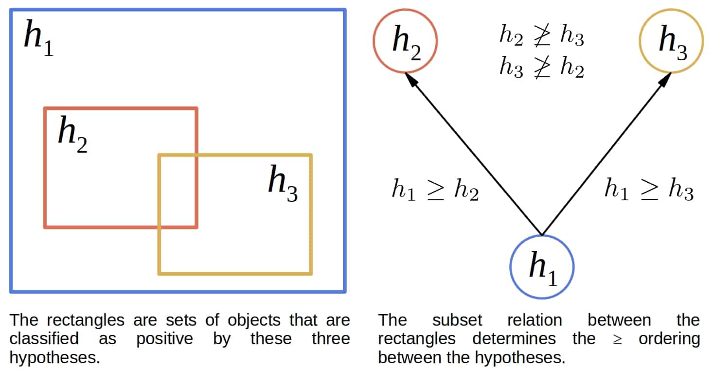
The most general hypothesis is the one that labels all examples as positive. Similarly, the most specific is the one that always returns  . The accompanying relations:
  (strictly more general),
  (strictly less general, strictly more specific), and
  are analogously defined. For brevity, we’ll refer to as “more general than” from now on.
4.2. Finding the Version Space
CEA finds the version space  by identifying its general and specific boundaries,
  and
and  .
.  contains the most general hypotheses in
  , whereas the most specific ones are in
  . We can obtain all the hypotheses in by specializing the ones from until we reach or by generalizing those from until we get .
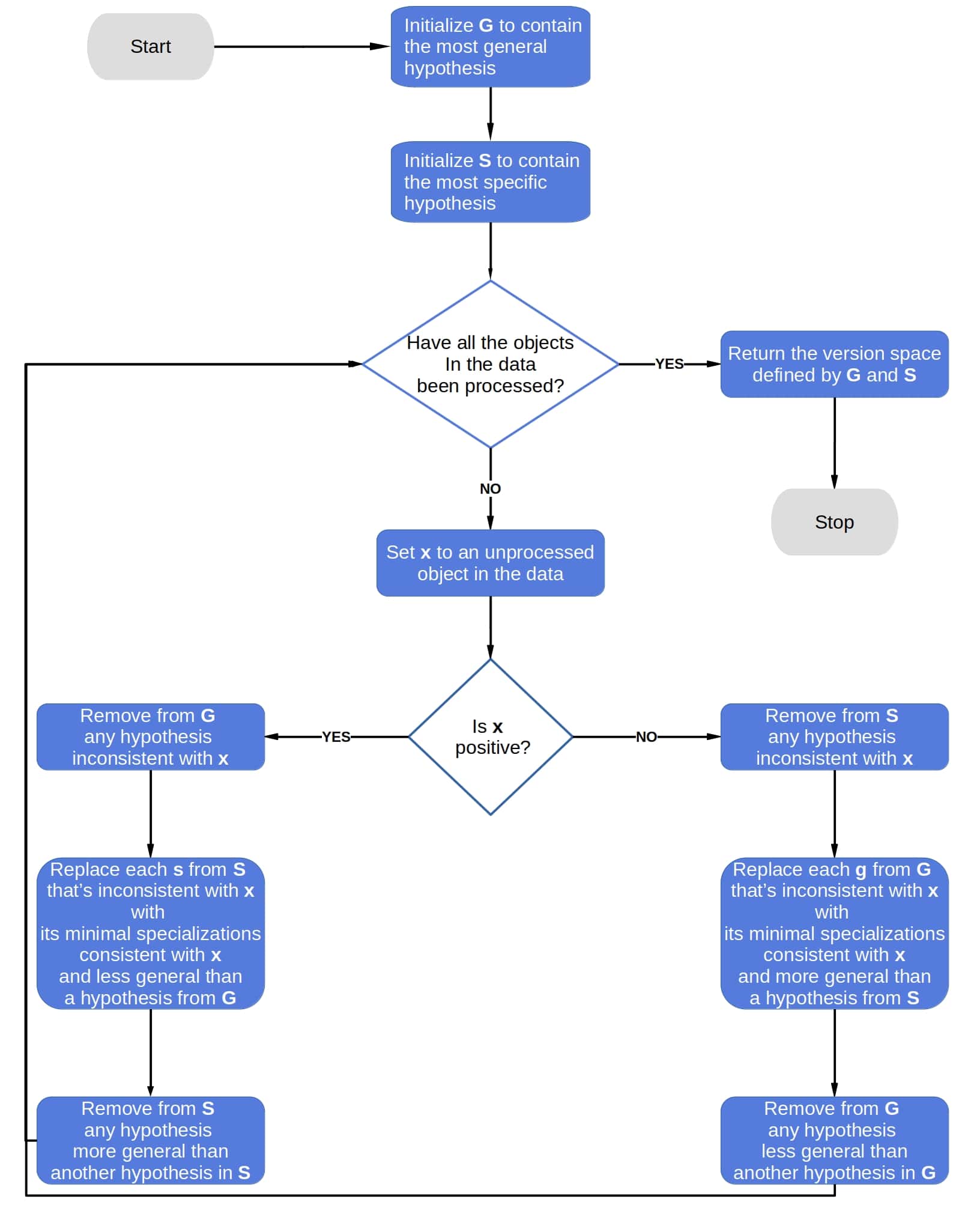
Let’s denote as  the version space whose general and specific boundaries are and . At the start of CEA, contains only the most general hypothesis in
  . Similarly, contains only the most specific hypothesis in . CEA processes the labeled objects one by one. If necessary, it specializes and generalizes so that the
  correctly classifies all the objects processed so far:
algorithm CandidateElimination(D):
    // INPUT
    //    D = a dataset of objects labeled as positive or negative
    // OUTPUT
    //    V = the version space of hypotheses consistent with D

    Initialize G to the set containing the most general hypothesis
    Initialize S to the set containing the most specific hypothesis

    for each object x in D:
        if x is a positive object:
            Remove from G any hypothesis inconsistent with x
            for each hypothesis s in S that is inconsistent with x:
                Remove s from S
                Add to S all the minimal generalizations h of s such that h is consistent with x
                  and for some member g of G it holds that g >= h
                Remove from S any hypothesis that is more general than another hypothesis in S
        else:
            Remove from S any hypothesis inconsistent with x
            for each hypothesis g in G that is inconsistent with x:
                Remove g from G
                Add to G all the minimal specializations h of g such that h is consistent with x
                  and for some member s of S it holds that h >= s
                Remove from G any hypothesis that is less general than another hypothesis in G

    return V as V(G, S)
5. An Example of CEA in Practice
Let’s show how CEA would handle the example with our friend Aldo.
5.1. Initialization
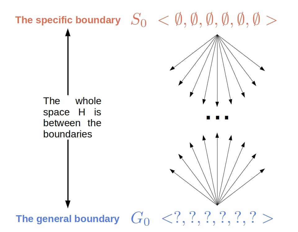
In the beginning, CEA initializes to  and to
  . The space bounded by
  and
and  ,
,  , is the whole hypothesis space :
5.2. Processing the First Positive Object
Since the only hypothesis in ,  , is consistent with the object
  , CEA doesn’t change the general boundary in the first iteration, so it stays the same:
  .
.
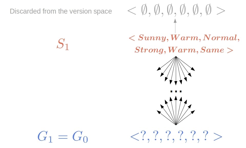
However,  as the only hypothesis in is not consistent with the object, so we remove it. The minimal generalization of that covers the object is precisely the hypothesis . It’s less general than the hypothesis in
  . So, the updated specific boundary is
  :
:
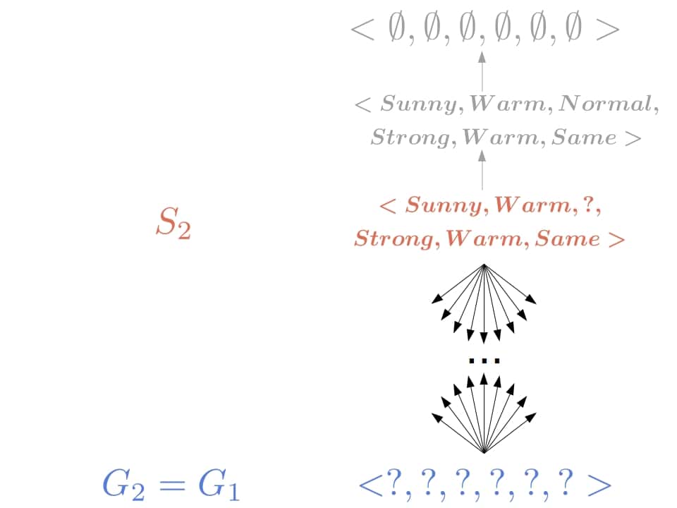
5.3. Processing the Second Positive Object
As the hypothesis is consistent with the positive example  , no changes to the general boundary are necessary. So, it will hold that
  .
.
However, hypothesis from  is overly specific, so we remove it from the boundary. Its minimal generalization that covers the second positive object is
  , which is less general than we have in
  , so
, so  :
:
5.4. Processing the First Negative Object
The third example in our data ( ) is negative, so we execute the else-branch in the main loop of CEA. Since
  is not inconsistent with the object, we don’t change it, so we’ll have
  . Inspecting , we see that is too general and remove it from the boundary. Next, we see that there are six minimal specializations of the removed hypothesis that are consistent with the example:
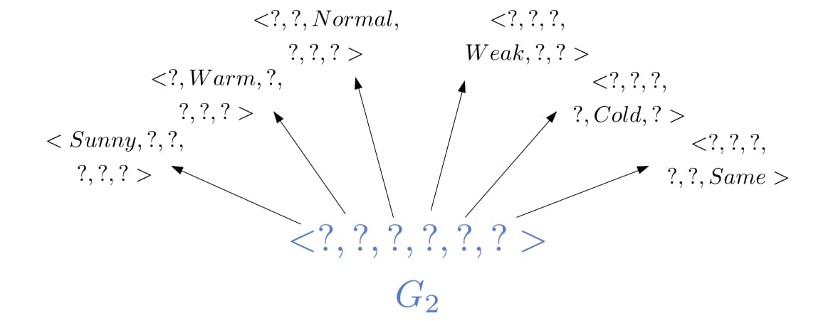
To specialize a hypothesis so that it correctly classifies a negative object, we replace each  in the hypothesis with values other than the one in the object. So, we have
  instead of
  ,
,  instead of
  , and so on.
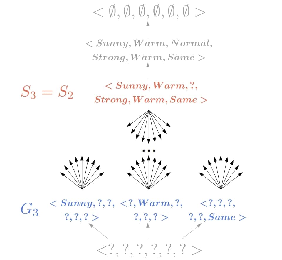
However, only  ,
,  , and
, and  are more general than the hypothesis we have in
  . A hypothesis that isn’t more general than at least one hypothesis in the specific boundary doesn’t classify all the positive examples as positive. That’s why we keep only the minimal specializations that are than the hypothesis in :
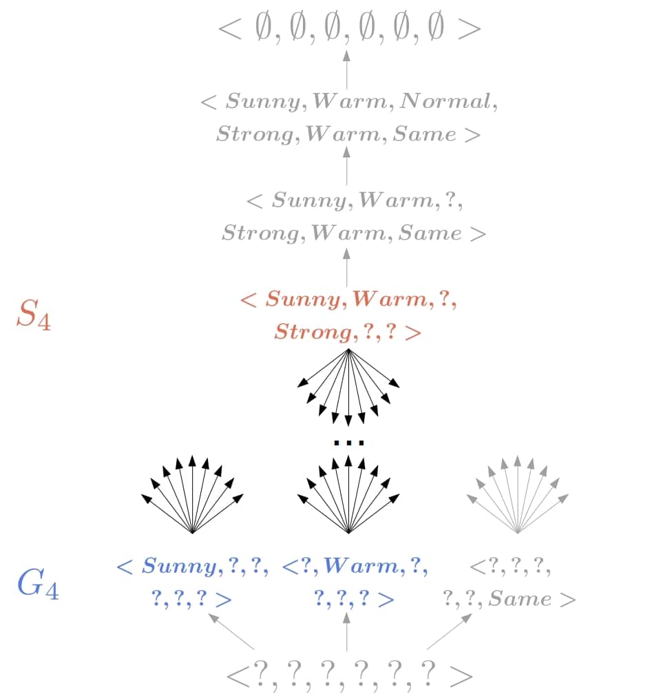
5.5. Processing the Third Positive Object
Since the hypothesis  is inconsistent with the object
  , we remove it. We can’t specialize it because all its specializations wouldn’t classify the object as positive. Similarly, we can’t generalize it as that wouldn’t be consistent with the negative object we previously processed. Therefore, the only option is to remove the hypothesis.
The object shows that is overly specific, so CEA generalizes the hypothesis in to  , and we get a new boundary
  .
.
Finally, CEA returns the version space  :
:
6. Convergence of CEA
If contains a hypothesis that correctly classifies all the training objects and the data have no errors, then the version space CEA finds will include that hypothesis. If the output version space contains only a single hypothesis  , then we say that CEA converges to . However, if the data contain errors or doesn’t contain any hypothesis consistent with the whole dataset, then CEA will output an empty version space.
7. Speeding up CEA
The order in which CEA processes the training objects doesn’t affect the resulting version space, but it affects the convergence speed. CEA attains the maximal speed when it halves the size of the current version space in each iteration, as that reduces the search space the most.
A good approach is to allow CEA to query the user for a labeled object to process next. Since CEA can inspect its version space, it can ask for an object whose processing would halve the space’s size.
8. Partially Learned Concepts
If the version space contains multiple hypotheses, then we say that CEA has partially learned the target concept. In that case, we must decide how to classify new objects.
One strategy could be to classify a new object  only if all the hypotheses in agree on its label. If there’s no consensus, we don’t classify . An efficient way of doing so is to consider the space’s boundaries and . If all the hypotheses in classify as positive, then we know that all the other hypotheses in will too. That’s because they’re all at least as general as those in . Conversely, we may test if the hypotheses in agree that is negative. Hence, there’s no need to look beyond the boundaries if we seek unanimity.
On the other hand, if we can tolerate disagreement, then we can output the majority vote. If we take all the hypotheses in to be equally likely, then the majority vote represents the most probable classification of . Additionally, the percentage of hypotheses classifying as positive can be considered the probability that is positive. The same goes for negative classification.
9. Unrestricted Hypothesis Spaces
If contains no hypothesis consistent with the dataset, then CEA will return an empty version space. To prevent this from happening, we can choose a representation that makes any concept a member of . If  is the space the objects come from, then should represent every possible subset of . In other words, should correspond to the power set of .
One way to do that is to allow complex hypotheses that consist of disjunctions, conjunctions, or negations of simpler hypotheses. To do so, we’d first design atomic hypotheses, which are the simplest of all. For instance, we’d say that the definition of hypotheses we gave in Section 3 describes the atomic hypotheses in our working example. Then, we’d add two more rules to allow combinations:
- The atomic hypotheses are hypotheses.
- If and are hypotheses, then
 ,
,  , and
, and  are also hypotheses.
9.1. Overfitting the Data
But, the problem is that a so expressive space will cause CEA to overfit the data! The returned version space’s specific boundary will memorize all the positive training objects ( ), whereas its general boundary will memorize all the observed negative instances (
 ):
):
![\[\begin{aligned} S &=&& \left\{\left(\bigvee_{x \in D^+}x\right)\right\} \\ G &=&& \left\{\neg \left(\bigvee_{x\in D^-}x\right)\right\} \end{aligned}\]](/wp-content/ql-cache/quicklatex.com-501ab820afbd3e018550d04800ea1d76_l3.svg "Rendered by QuickLaTeX.com")
9.2. Classification in Unrestricted Spaces
As a result, such a version space provides the unanimous vote only when asked about the training objects. For any other object , half the hypotheses in  classify it as positive, while the other half classifies it as negative. Since corresponds to the power set of , we know that for any
  that classifies as positive, there must be an
  that agrees with on all the objects except for , which it labels as negative. But since and
  disagree only on a non-training object, is also in . So, unrestricted hypothesis spaces are useless, and some sort of restriction is necessary.
10. From Inductive Bias to Deductive Reasoning
That restriction biases the search towards a specific type of hypothesis and is therefore called the inductive bias. We can describe bias as a set of assumptions that allow deductive reasoning. That means that we can prove that the version spaces output correct labels. Essentially, we regard the labels as theorems and the training data, the object to classify, and the bias as the input to a theorem prover.
If we require the unanimous vote of hypotheses in a version space, then the inductive bias of CEA is simply:
The hypothesis space contains the target concept.
That’s the weakest assumption we’d have to adopt in order to have formal proofs for labels. However, we should note that the proofs will be semantically correct only if the bias truly holds.
11. Conclusion
In this article, we explained the Candidate Elimination Algorithm (CEA). We showed how to use it for concept learning and also discussed its convergence, speed, and inductive bias.