Difference between Big-O and Little-o Notations

1. Overview

In this brief tutorial, we’ll learn about how big-O and little-o notations differ. In short, they are both asymptotic notations that specify upper-bounds for functions and running times of algorithms.

However, the difference is that big-O may be asymptotically tight while little-o makes sure that the upper bound isn’t asymptotically tight.

Let’s read on to understand what exactly it means to be asymptotically tight.

2. Mathematical Definition

Big-O and little-o notations have very similar definitions, and their difference lies in how strict they are regarding the upper bound they represent.

2.1. Big-O

For a given function $g(n)$ , $O(g(n))$ is defined as:

$O(g(n)) = \{f(n):$ there exist positive constants $c$ and $n_0$ such that $0 \le f(n) \le cg(n)$ for all $n \ge n_0\}$ .

So $\pmb{O(g(n))}$ is a set of functions that are, after $\pmb{n_0}$ , smaller than or equal to $\pmb{g(n)}$ . The function’s behavior before $n_0$ is unimportant since big-O notation (also little-o notation) analyzes the function for huge numbers. As an example, let’s have a look at the following figure:

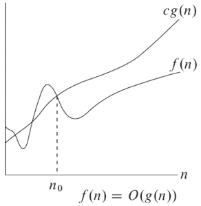
Here, $f(n)$ is only one of the possible functions that belong to $O(g(n))$ . Before $n_0$ , $f(n)$ is not always smaller than or equal to $g(n)$ , but after $n_0$ , it never goes above $g(n)$ .

The equal sign in the definition represents the concept of asymptotical tightness, meaning that when $\pmb{n}$ gets very large, $\pmb{f(n)}$ and $\pmb{g(n)}$ grow at the same rate. For instance, $3n^3 = O(n^3)$ satisfies the equal sign, hence it is asymptotically tight, while $3n = O(n^3)$ is not.

For more explanation on this notation, look at an introduction to the theory of big-O notation.

2.2. Little-o

Little-o notation is used to denote an upper-bound that is not asymptotically tight. It is formally defined as:

$o(g(n)) = \{f(n):$ for any positive constant $c$ , there exists positive constant $n_0$ such that $0 \le f(n) < cg(n)$ for all $n \ge n_0\}$ .

Note that in this definition, the set of functions $\pmb{f(n)}$ are strictly smaller than $\pmb{cg(n)}$ , meaning that little-o notation is a stronger upper bound than big-O notation. In other words, the little-o notation does not allow the function $f(n)$ to have the same growth rate as $g(n)$ .

Intuitively, this means that as the $n$ approaches infinity, $f(n)$ becomes insignificant compared to $g(n)$ . In mathematical terms:

$\lim_{n\to\infty} \frac{f(n)}{g(n)} = 0$

In addition, the inequality in the definition of little-o should hold for any constant $c$ , whereas for big-O, it is enough to find some $c$ that satisfies the inequality.

If we drew an analogy between asymptotic comparison of $f(n)$ and $g(n)$ and the comparison of real numbers $a$ and $b$ , we would have $f(n) = O(g(n)) \approx a \le b$ while $f(n) = o(g(n)) \approx a < b$ .

3. Examples

Let’s have a look at some examples to make things clearer.

For $f(n) = 2n + 3$ , we have:

$\pmb{f(n) = O(n)}$ but $\pmb{f(n) \ne o(n)}$
$f(n) = O(n^2)$ and $f(n) = o(n^2)$
$f(n) = O(n^3)$ and $f(n) = o(n^3)$

In general, for $f(n) = a_xn^x + a_{x-1}n^{x-1} + ... + a_0$ , we will have:

$\pmb{f(n) = O(n^x)}$ but $\pmb{f(n) \ne o(n^x)}$
$f(n) = O(n^{x+1})$ and $f(n) = o(n^{x+1})$
$f(n) = O(n^{x+2})$ and $f(n) = o(n^{x+2})$

For more examples of big-O notation, see practical Java examples of the big-O notation.

4. Conclusion

In this article, we learned the difference between big-O and little-o notations and noted that little-o notation excludes the asymptotically tight functions from the set of big-O functions.

Full Archive

About Baeldung

Core Concepts

Operating Systems

Artificial Intelligence

Graph Theory

Latex