

Learn through the super-clean Baeldung Pro experience:
>> Membership and Baeldung Pro.
No ads, dark-mode and 6 months free of IntelliJ Idea Ultimate to start with.
Learn through the super-clean Baeldung Pro experience:
>> Membership and Baeldung Pro.
No ads, dark-mode and 6 months free of IntelliJ Idea Ultimate to start with.
The best-first search is a class of search algorithms aiming to find the shortest path from a given starting node to a goal node in a graph using heuristics. The AO* algorithm is an example of the best-first search class. In this tutorial, we’ll discuss how it works.
This class should not be mistaken for breadth-first search, which is just an algorithm and not a class of algorithms. Moreover, the best-first search algorithms are informed, which means they have prior knowledge about the distances from heuristics. However, the breadth-first search algorithm is uninformed.
The AO* algorithm is based on AND-OR graphs to break complex problems into smaller ones and then solve them. The AND side of the graph represents those tasks that need to be done with each other to reach the goal, while the OR side stands alone for a single task. Let’s see an example below:
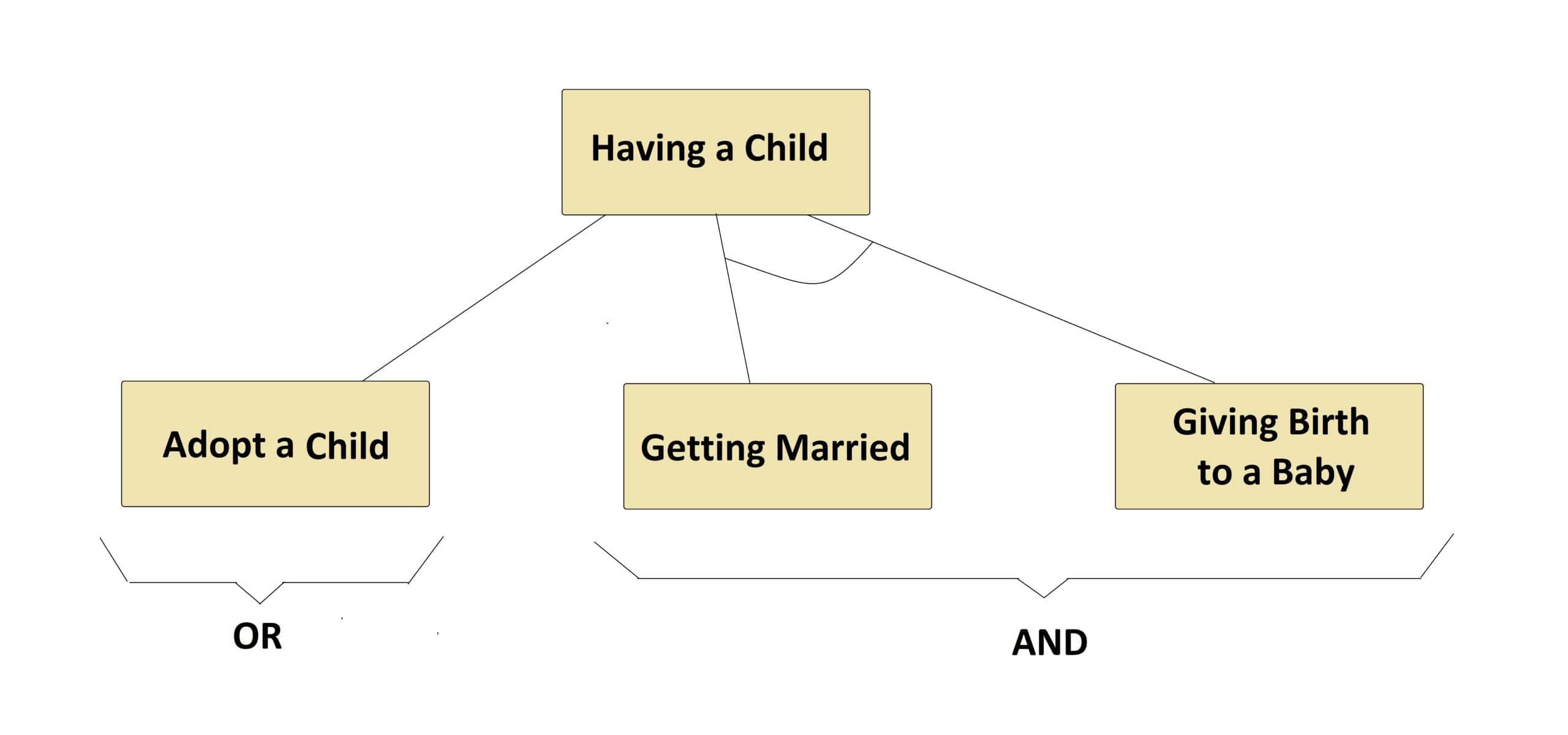
In the above example, we can see both tasks of the AND side, which are connected by an AND-ARCS, need to be done to have a child, while the OR side lets having a child just by a single task of adoption.
In general, in a graph for each node, there could be multiple OR and AND sides, where each AND side itself may have multiple successor nodes connected to each other by an AND-ARCS.
AO* works based on this formula:  , where
  is the actual cost of going from the starting node to the current node,
  is the estimated or heuristic cost of going from the current node to the goal node, and
  is the actual cost of going from the starting node to the goal node.
Let’s see an example below to explain AO* step by step to find the lowest cost path from the starting node  to the goal node:
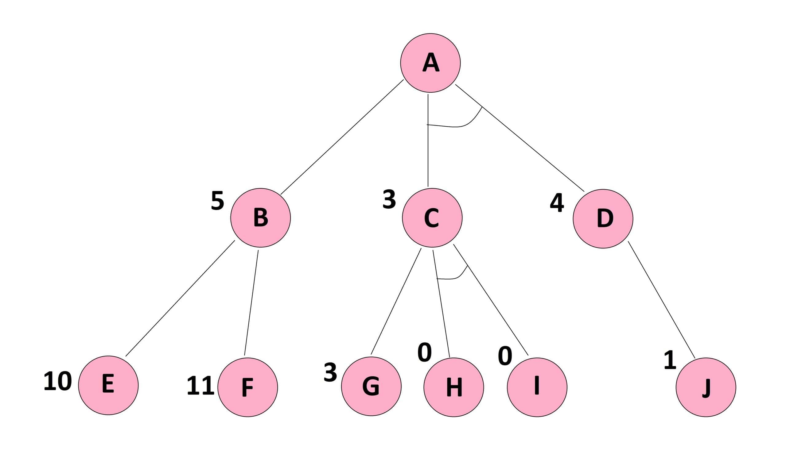
It should be noted that the cost of each edge is the same as  , and the heuristic cost to reach the goal node from each node of the graph is shown beside it.
Moreover, it is worth mentioning that we may not see the goal node in this graph, but it does not matter because we already know the heuristic costs from each node of this graph to that unseen goal node.
First, we begin from node and calculate each of the OR side and AND side paths. The OR side path  , where is the cost of the edge between and
  , and
, and  is the estimated cost from to the goal node.
The AND side path  , where the first is the cost of the edge between and
  ,
,  is the estimated cost from to the goal node, the second is the cost of the edge between and
  , and
, and  is the estimated cost from to the goal node. Let’s see an example below:
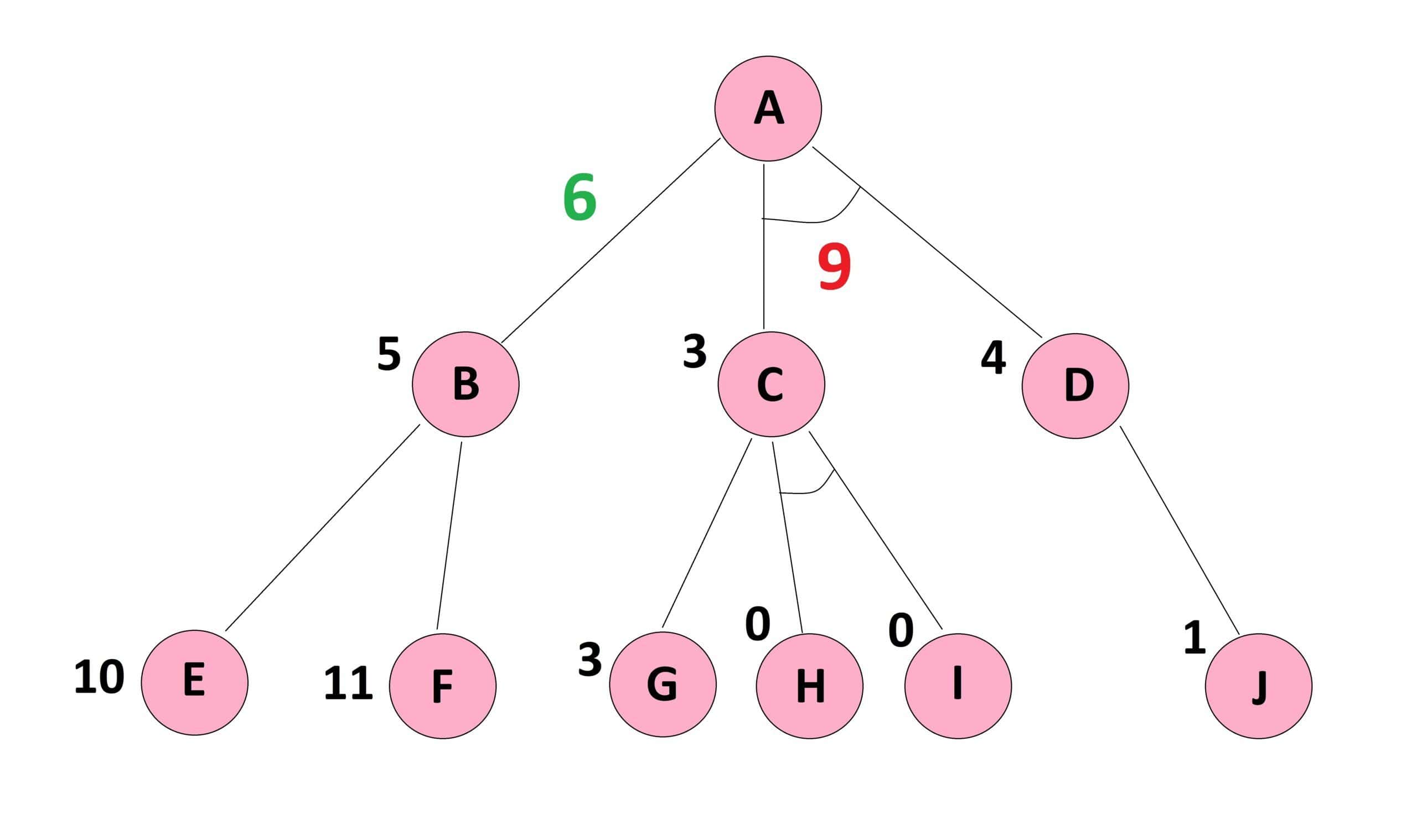
Since the cost of  is the minimum cost path, we proceed on this path in the next step.
Here, someone may ask why we do not stop here since we have already found the minimum cost path from to the goal node. The answer is that such a path may not be the correct minimum cost path because we have made our calculations based on the heuristics down to only one level. However, the given graph has provided us with a deeper level whose calculations may update the achieved values.
In this step we continue on the from to its successor nodes i.e.,  and
and  , where
  and
and  . Here,
  has a lower cost and would be chosen.
Now, we have reached the bottom of the graph where no more level is given to add to our information. Therefore, we can do the backpropagation and correct the heuristics of upper levels. In this vein, the updated  , and as a consequence the updated
  . Let’s see an example below:
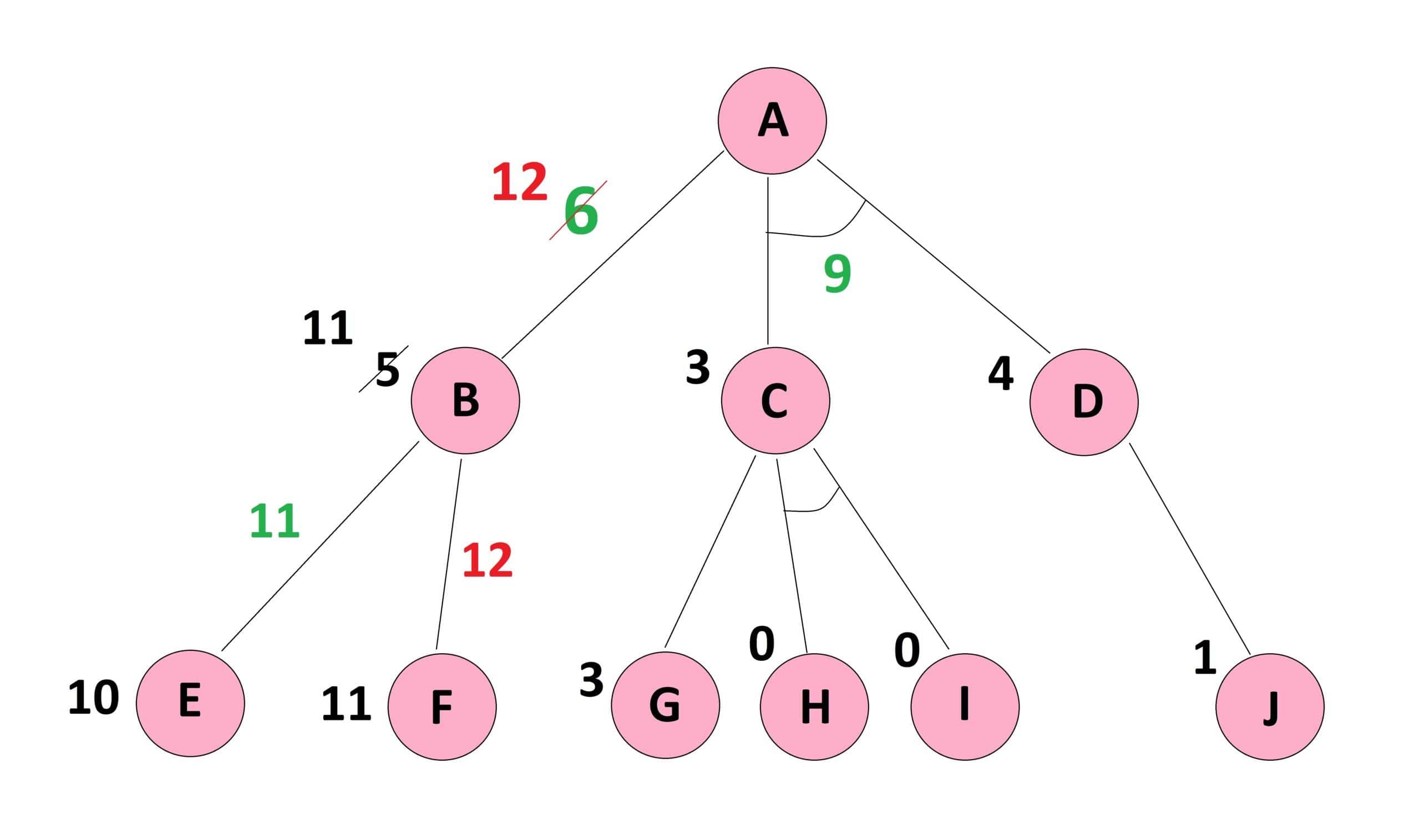
Now, we can see that  with a cost of
  is lower than the updated with a cost of
  . Therefore, we need to proceed on this path to find the minimum cost path from to the goal node.
It is worth mentioning that if the updated had a lower cost than , then we were done, and no more calculations would be required.
In this step, we do the calculations for the AND side path, i.e., , and first explore the paths attached to node . In this node again we have an OR side where  , and an AND side where
  , and as a consequence the updated
  .
.
Also, the updated  , since
  . By these updated values for
  and
and  , the updated
  . Let’s see an example below:
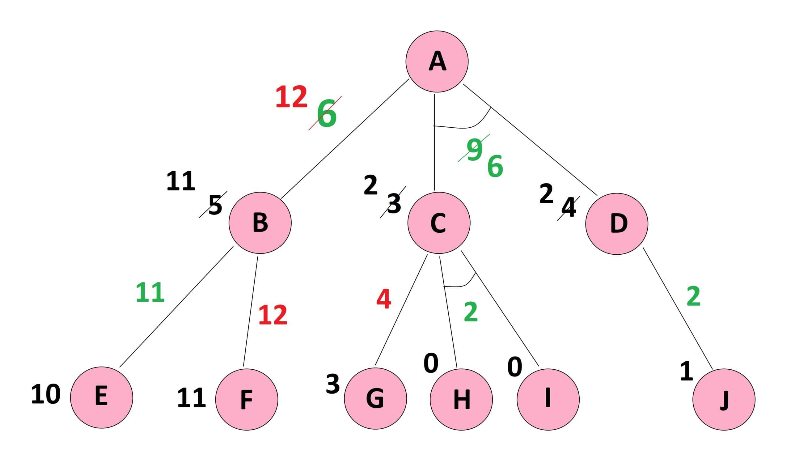
This updated with the cost of  is still less than the updated with the cost of , and therefore, the minimum cost path from to the goal node goes from by the cost of . We are done.
In this section, we present the pseudocode of the AO* algorithm. As we have seen in the above example, the process goes into a cycle of forward and backward propagation until there is no more change in the minimum cost path. To simplify, we did not go into details of the backpropagation since it follows the same rules of forward propagation but in the opposite direction. Let’s see the pseudocode below:
algorithm AOStar(Graph, StartNode):
    // INPUT
    //    Graph = the graph to search
    //    StartNode = the starting node
    // OUTPUT
    //    The minimum cost path from StartNode to GoalNode

    CurrentNode <- StartNode

    while there is a new path with lower cost from StartNode to GoalNode:
        calculate the cost of path from the current node to the goal node
          through each of its successor nodes

        if the successor node is connected to other successor nodes by AND-ARCS:
            sum up the cost of all paths in the AND-ARC
            return the total cost
        else:
            calculate the cost of the single path in the OR side
            return the single cost

        find the minimum cost path

        CurrentNode <- Successor Node Of Minimum Cost Path

        if CurrentNode has no successor node:
            do the backpropagation and correct the estimated costs
            CurrentNode <- StartNode
            return CurrentNode, New estimated costs
        else:
            return null

return The minimum cost pathThe AO* algorithm is not optimal because it stops as soon as it finds a solution and does not explore all the paths. For example, if the early heuristic value of were more than , we would never explore this side, and the solution remained for the OR side.
However, AO* is complete, meaning it finds a solution, if there is any, and does not fall into an infinite loop. Moreover, the AND feature in this algorithm reduces the demand for memory.
The space complexity comes in polynomial order, while the time complexity is  , where
  stands for branching and
  is the maximum depth or number of levels in the search tree.
In this tutorial, we examined AO* as a sample of best-first search algorithms. We noticed that the strength of this algorithm comes from a divide and conquer strategy. The AND feature brings all the tasks of the same goal under one umbrella and reduces the complexities. However, such a benefit comes at the cost of losing optimality.