Ant Lion Optimization | Baeldung on Computer Science

1. Introduction

Inspired by nature, the Ant Lion Optimizer gives us a meta-heuristic algorithm for optimization problems. It is a population-based algorithm. The populations we focus on are antlions and ants. Antlions in their larval form hunt ants by digging pits in the sand, which can cause the ant to fall towards the center where the antlion is waiting to strike. Antlions are complemented by exploratory ants acting as search agents.

2. Representing the World

Our world contains two entities, ants and antlions. We need to model them and their behavior. In order to do that, we use vectors to represent antlions and ants and matrices for populations of the same. The behavior we model is the random walk of ants and the effect of antlion traps on those walks. By updating antlion positions to good ant positions, the algorithm converges to an optimal solution over time.

2.1. Representing Ants

Ants are search agents that randomly walk through the space. We score ants using a fitness function as they walk between antlion traps.

Ants move through the world using a stochastic policy. We use a random walk. The goal for the ants is to avoid the antlions.

The random walk of an ant is computed using the following equation:

(1) $\begin{equation*} X(t) = [0,cumsum(2r(t_1)-1),cumsum(2r(t_1)-1),..,cumsum(2r(t_n)-1)] \end{equation*}$

In this case $cumsum$ is the cummulative sum function. We also use a random function $r(t)$ which we show below:

(2) $\begin{equation*} r(t) = \begin{cases} 1, & \text{if}\ rand > .5 \\ 0, & \text{if}\ rand \leq .5 \end{cases} \end{equation*}$

Rand is a random number sampled uniformly from the range $[0,1]$

In the image below we show the result of 3 random walks in one-dimension through time. The walks rise and fall above and below the origin quite dramatically in some cases. This will allow for a good level of exploration around existing solutions:

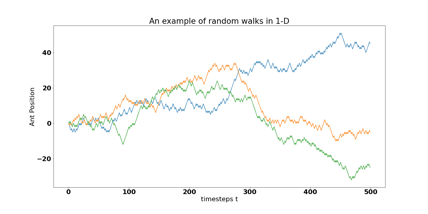
We will revisit the random walk described here in order to bound it and integrate its behavior with the existence of antlions. We first introduce antlions.

2.2. Representing Antlions

The goal for the antlions is to capture ants. Antlions represent solutions to the optimization problem. We represent antlions with a matrix. Antlions dig pits, which act as traps, into which ants can stumble. In this way, antlions affect the random walk of ants. We model this behavior by having the random walk of the ants affected by the antlions.

The random walk of ants, modelled to include the effect of antlion traps is shown below:

(3) $\begin{equation*} X_{i}^{t} =\frac{(X_{i}^{t} - a_i)\times (d_i - c_{i}^{t})}{b_{i}^{t} - a_i} + c_i \end{equation*}$

In the random walk equation above, we are normalizing the ant’s position. Here we represent the minimum value of the random walk along dimension $i$ as $a_{i}$ and the maximum value along dimension $i$ as $b_{i}$ . This is a normal min-max scaling. We extend this scaling to include the effect of antlion traps.

(4) $\begin{equation*} c_{i}^{t} = \text{Antlion}_{j}^{t} + c^{t} \end{equation*}$

(5) $\begin{equation*} d_{i}^{t} = \text{Antlion}_{j}^{t} + d^{t} \end{equation*}$

These normalization terms are used to keep the random walk within the bounds of a chosen antlion trap, by decreasing the bounds overtime we can achieve the effect of trapping an ant. This impacts the dynamics of the walk itself. If an ant enters a trap, the antlion attempts to knock it towards the center of the pit.

Elitism is also used through storing the best performing antlion and allowing it to affect all other searches. We achieve this by having ants walk within two antlion pits and average between them. The best performing antlion and an antlion are chosen via a roulette wheel. Better performing antlions are more likely to be chosen.

By roulette wheel, we mean using weighted random selection. The selection is biased towards fitter antlions.

2.3. Trapping Ants

An ant is knocked towards the center of a trap by reducing the hypersphere an ant can explore around the trap. This is achieved through applying a ratio to the lower and upper bounds of the ant’s orbit. We will decay the size over time.

(6) $\begin{equation*} c^{t} = \frac{c^{t}}{Z} \end{equation*}$

(7) $\begin{equation*} d^{t} = \frac{d^{t}}{Z} \end{equation*}$

$Z$ is a ratio represented as $Z = 10^{w}\frac{t}{T}$ . In this equation $w$ is a constant for a given time interval and increased in a stepwise fashion. In this way $w$ allows us to control the amount of exploitation that takes place.

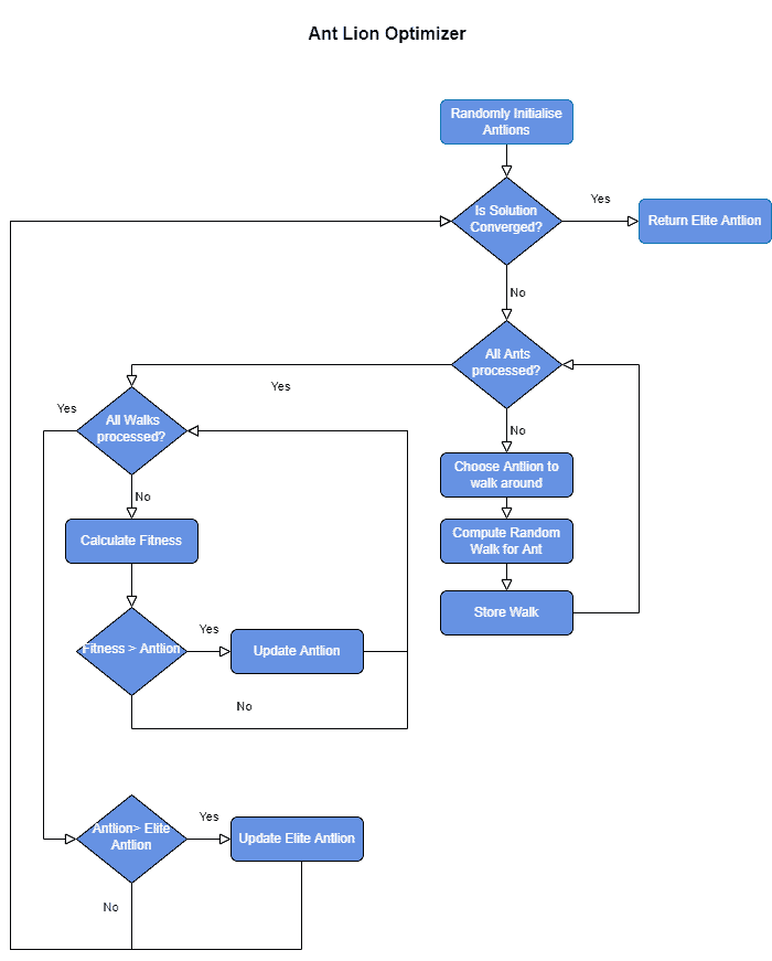
3. Algorithm Flow Chart

Before putting all the steps together, we present a flowchart for the algorithm. The flow chart shows the high-level description of the algorithm combining the operations we outlined above. The algorithm flows with a standard outer loop checking for a termination condition, e.g., Max number of iterations reached or algorithm converged. The inner loop computes each of the ant’s random walks. Once all the walks are computed, we can update the antlion positions where an ant became fitter than an antlion. If any antlion becomes better than our best elite antlion, then we update our elite antlion too:

Ant Lion Optimiser Described as a flow chart

4. Method

Let us put together all the behavior we have just modeled.

We start with a random population of antlions (solutions). Ants are then used to explore the space using random walks. These random walks lie within a bounded region, and they are affected by proximity to antlions.

This is modelled by reducing the hypersphere an ant can explore around an antlion over time. We model this with the lower bound $c_{i}^{t}$ and the upper bound $d_{i}^{t}$ . When an ant is caught and becomes fitter than its corresponding antlion, the antlion updates its position in order to optimize its chances of catching more ants. Over time the best antlions will converge to an optimal solution.

Elitism is used here to direct the search around good solutions. An ant’s random walk takes place around two antlions. The first antlion is chosen in a roulette wheel fashion, proportional to its fitness. The second is the elite antlion, the solution with the highest fitness discovered so far. The two proposed walks of the ant are averaged together.

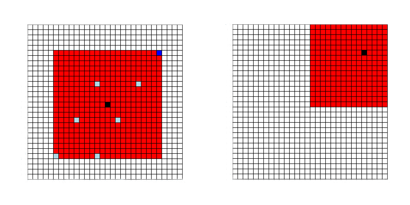
5. Example

For a single ant and antlion, we show a discrete random walk. The red tiles are the area covered by the antlions trap, which constrains the ants’ movement, and will be decreased over time. The black tile is the antlions’ current position. The light blue represents the tiles visited by the ant on its random walk and the dark blue is the final tile for this timestep. If the ant’s final position has a better fitness value than the current antlion, then the antlion repositions itself, and its trap, as shown in the second figure. Normally we would average the ant’s position with a corresponding random walk around a second elite antlion. This helps to expand the search into the world, white grid, not covered by the antlions trap:

An example of an ants walk within an antlions trap. The subsequent repositioning of the antlion once the ants fitness is better than the antlions.

6. Conclusion

ALO is a sound algorithm. The random walk of ants allows for a high degree of exploration. Local optima are avoided as ALO is a population-based algorithm making getting stuck in a local optimum unlikely. The random walks of ants and the roulette wheel selection of antlions help avoid stagnating in local optima. Exploitation is also encouraged through the shrinking of antlion trap boundaries, and the intensity of ant movements decreases over time, allowing for convergence.

The Ant Lion Optimizer is an easy-to-use, gradient-free, black-box optimization method. It is easy to use due to the few available tuneable parameters. It can be applied to various optimization problems and is part of a family of optimization methods, such as Moth Flame Optimization and Gray Wolf Optimization, which are a great addition to the optimization toolbox.

Full Archive

About Baeldung

Core Concepts

Operating Systems

Artificial Intelligence

Graph Theory

Latex