

Learn through the super-clean Baeldung Pro experience:
>> Membership and Baeldung Pro.
No ads, dark-mode and 6 months free of IntelliJ Idea Ultimate to start with.
Learn through the super-clean Baeldung Pro experience:
>> Membership and Baeldung Pro.
No ads, dark-mode and 6 months free of IntelliJ Idea Ultimate to start with.
In this tutorial, we’ll discuss three popular data types: list, queue, stack. Then, we’ll present the variation of each ADT, basic operations, and implementation strategy using data structures.
Data types are used to define or classify the type of values a variable can store in it. Moreover, it also describes the possible operations allowed on those values. For example, the integer data type can store an integer value. Possible operations on an integer include addition, subtraction, multiplication, modulo.
Abstract data type (ADT) is a concept or model of a data type. Because of ADT, a user doesn’t have to bother about how that data type has been implemented. Moreover, ADT also takes care of the implementation of the functions on a data type. Here, the user will have predefined functions on each data type ready to use for any operation.
Generally, in ADT, a user knows what to do without disclosing how to do it. These kinds of models are defined in terms of their data items and associated operations.
In every programming language, we implement ADTs using different methods and logic. Although, we can still perform all the associated operations which are defined for that ADT irrespective of language. For example, in C, ADTs are implemented mostly using structure. On the other hand, in C++ or JAVA, they’re implemented using class. However, operations are common in all languages.
ADTs are a popular and important data type. Generally, ADTs are mathematical or logical concepts that can be implemented on different machines using different languages. Furthermore, they’re very flexible and don’t dependent on languages or machines.
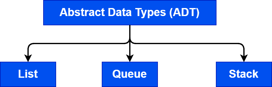
There are mainly three types of ADTs:
A list is an ordered collection of the same data type. Moreover, a list contains a finite number of values. We can’t store different data types in the same list. Here, ordered doesn’t mean that the list is sorted, but they’re properly indexed. Hence, if we know the location of the first element of a list, we can perform any operations on the whole list.
We can implement a list easily using an array. However, memory management is a big task for the implementation of a list using an array. In every programming language, we’ve to declare a fixed size for an array. Also, there is no significant maximum size that we can specify for an array. Hence, there’ll be a time when a list will overflow when implementing with an array. On the other hand, if we store fewer data, we can’t utilize the available memory efficiently.
To overcome this issue, we use structure or class to implement the list. As structure or class is dynamic, we’ll have the scope to add data to a run-time list.
There are three types of lists:
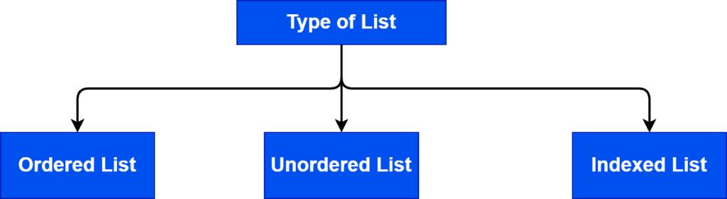
We store all the elements in ascending or descending order using the inherited characteristics of the elements in an ordered list. An example of an ordered list is a list ordered alphabetically or numerically.
In an unordered list, the elements are not sorted in any order from the characteristic of the elements. Hence, we’ll arrange the order of the elements according to the user’s convenience.
In an indexed list, elements are arranged, but their numeric positions are called indexes. Therefore, we can access elements from a list using indexes.
Let’s talk about the operations that can be performed on a list:
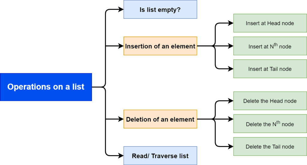
In a list, the basic operations are checking if a list is empty or not, inserting an element in some position, deleting an element from some position, and read the whole list. Let’s take a look at the functions:  ,
,  ,
,  ,
,  .
.
The function provides the information whether there is an element in the list or not. If there is no element in the list, it’s a null or empty list.
We use to insert elements at a given location in a list. Here,  denotes the position where we want to insert an element in a list.
To delete an element from a list, we use the function. Here denotes the position from where we want to delete an element in a list.
We use to read all the elements from a list.
Now let’s discuss the data structures that can be used to implement a list. Here, we’ll discuss how to implement a list using array and linked list data structure.
The first step of the implementation of a list using an array is we declare a fixed-size array. This implementation stores a list inside an array. We index the elements in the list between  and
and  . Here,
  denotes the number of elements in the list.
The main problem with the array implementation is that we need to declare the size in advance. For example, let’s take a one-dimensional array of length  . If the size of the array is full, we need to create an array of a bigger size. After that, we’re forced to free the memory which is occupied by the previous array:
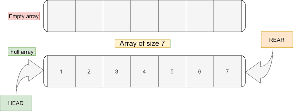
Now, this list is full. So if we need to add more elements, we’ve to create a bigger array and store the list in it.
In general, arrays are not a good choice for implementing lists. Moreover, the insertion and deletion with an array are expensive. Additionally, sometimes the size of the list is not known in advance.
The second choice to implement a list is using a dynamic data structure like a linked list. Although a list implemented using an array is simple but complex for memory management. We don’t have any provision to increase the size of the list at run time.
In linked list implementation, we can free and allocate the memory to a list in run time. Here, we divide each element into nodes. Moreover, each node stores the data and the address of the next node:
In this example,  is a pointer that stores the address of the first node. Furthermore, the address of the rear would be null as we don’t have to keep any address. If we know the address of the first node, we can perform all the operations on the list.
Accessing any element in the list will take constant time as each element has an index associated with it. Hence, the time complexity to access any element from the list is  . Also, the insertion and deletion of any element from the end of the list don’t depend on the size of the list. Therefore, insertion and deletion of any element from the end take constant time.
Insertion or deletion of an element at the head of the list can take time. Here, we need to shift all the elements proportional to the length of the list. So for that, time complexity would be  .
.
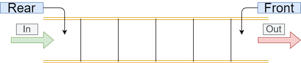
A queue is a linear ADT with the restriction that insertion can be performed at one end and deletion at another. It works on the principle of FIFO (first-in, first-out). Hence, the first element to be removed from the queue is the element added first. We can store only one data type in a queue.
There are two ends of a queue. One end is called the rear-end from where we can insert the data. The other end is the front-end from where we take out data from a queue:
We divide a queue into 4 types:
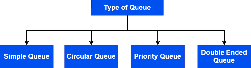
A simple queue is the simplest form of queue ADT. It inserts data from the rear end and removes elements from the front end. Moreover, a simple queue strictly obeys FIFO.
In a circular queue, the first element in the queue points to the last element in the queue, making it a circular structure. It utilizes memory in a better way compared to a simple queue.
A special queue named priority queue stores a priority for each element in the queue. A priority queue handles the removal and insertion operations based on the priority associated with each element.
A double-ended queue doesn’t obey the FIFO rule. We can insert and remove elements from both the rear and front ends.
Let’s explore the basic operations of a queue:
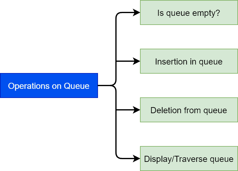
Here we’ll discuss some fundamental functions on a queue:  .
.
We use the function  to check if the queue is empty or not. The function
  insert a given value in the queue. We can’t add a value at any given location.
 remove an element from the queue. Similar to the insertion function, we can’t delete any element from a queue. It’s only allowed to delete elements from the front side of a queue.
 reads all the elements from a queue. It will read all values from front to rear of a queue.
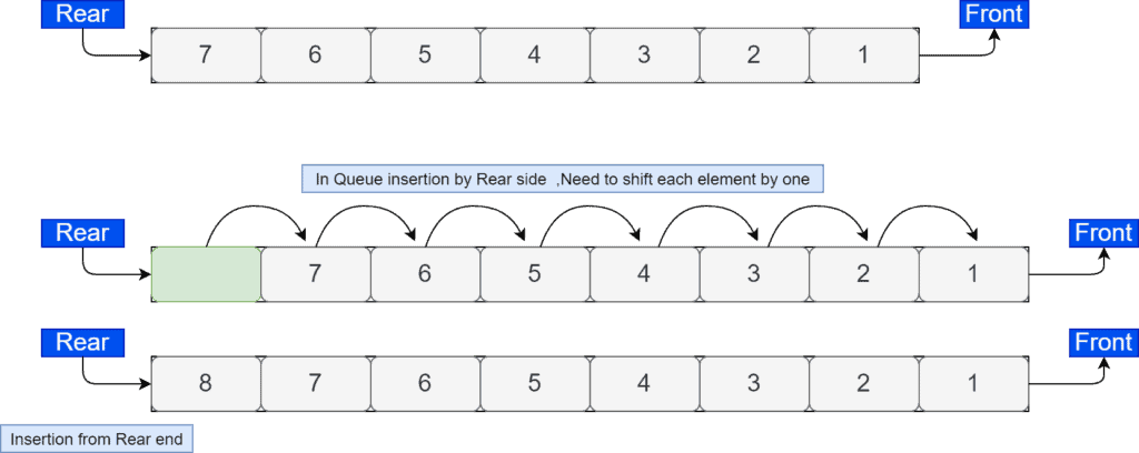
Implementation of a queue using an array is very simple. We just have to stick with the FIFO principle. Both insertion and deletion operations are allowed from either the front or rear end. In this implementation, we’ve to shift one element whenever we insert an element in an array. Initially, when the array is empty, the rear is  . We shift each element that is inserted in a queue from the rear end:
The major problem implementing a queue using an array is that it’ll only work when the size of the queue is known. Moreover, the size of the queue should be static.
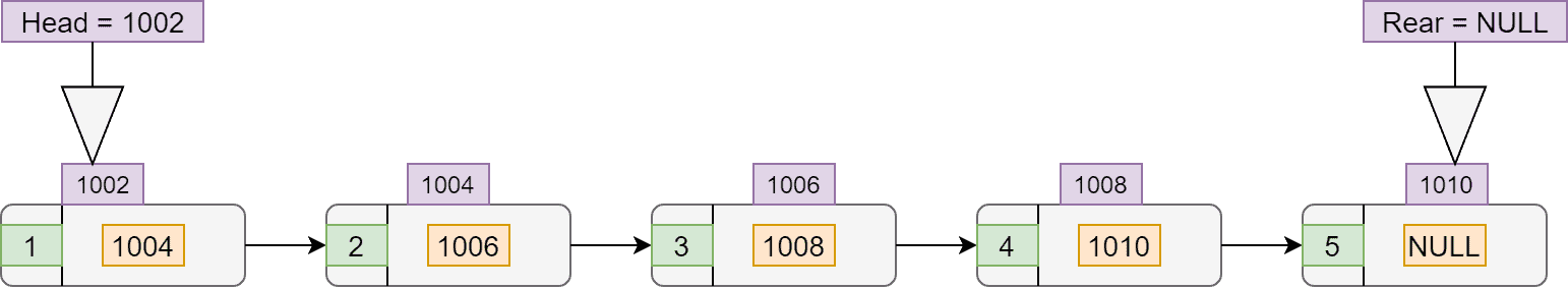
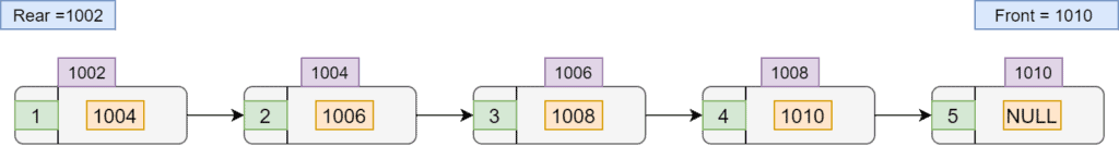
We can also implement a queue using a linked list data structure. In this implementation, there are nodes that store data and link for the next node, same as the implementation of the list using a linked list. The only difference is that we’re using two-pointers here. The rear stores the address of the last inserted element in the linked list. On the other hand, the front stores the address of the first inserted element in the linked list:
The time complexity for insertion and deletion in a queue is . Although, in order to search an element in a given queue takes time in the worst case.
Stack is a liner ADT, with restrictions in inserting and deleting elements from the same end. It’s like making a pile of plates in which the first plate will be the last plate to be taken. It works on the principle of LIFO (last-in, last-out). It stores only one type of data:
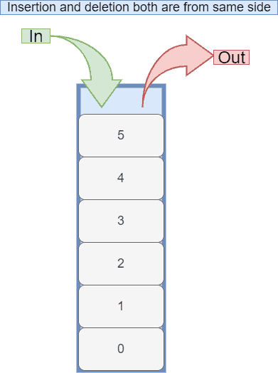
A stack has two core operations: push and pop. Push operation inserts a given element on the top of a stack. Pop operation removes the most recently added element from a stack.
A stack can be divided into 2 broad categories:
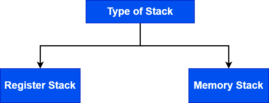
The register stack refers to a memory location generally on the CPU, which stores the addresses of the elements in the top region of a stack. It contains only a small amount of data compared to a stack.
The memory stack also refers to a memory location that stores a large amount of data compared to the memory stack. The depth of the stack in a memory register is flexible.
We’ll discuss 4 basic operations of a stack:
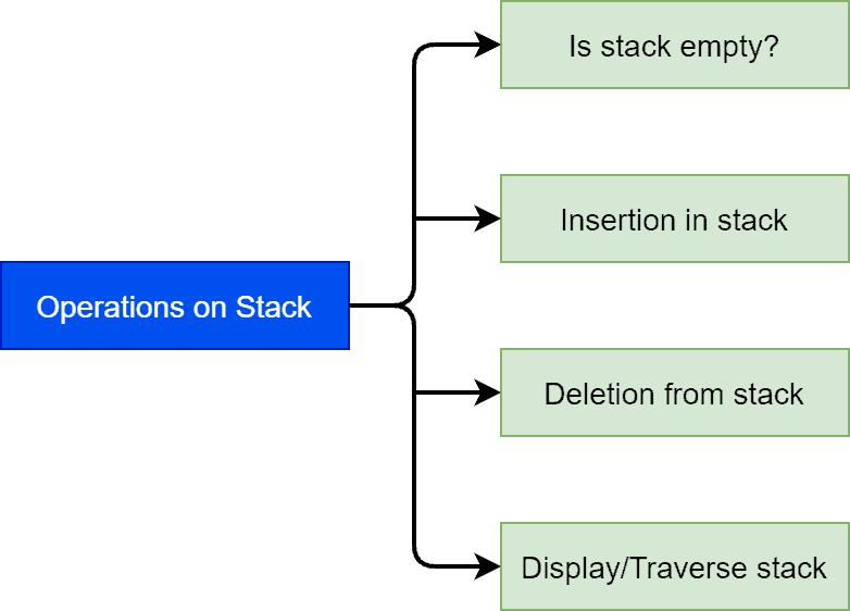
The function  is utilized to check if the stack is empty or not. We can use the function
  to insert a given element or value in a stack.
 will perform the deletion operation from a stack. In order to read all the element in a stack, we can use
  .
.
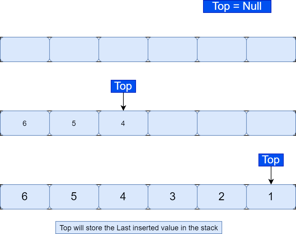
We can implement a stack using a one-dimensional array. The first step is to define the size of an array. Importantly, we need to follow the LIFO principle in order to insert or delete elements from an array. Additionally, we define a special variable  to store the data. Initially, when the stack is empty,
  is . Whenever we insert an element in a stack, stores the last inserted element:
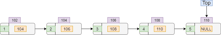
We can implement a stack using a linked list. Here we can increase the size of the stack at run time as we can allocate memory dynamically. There is a pointer for the variable that stores the address of the most recently added node. To delete an element from the stack, we emove the element pointed by the variable by pointing to the previous node of the linked list. Initially, when the stack is empty, points to null:
The time complexity of insertion and deletion of an element from the stack would be . Although if we want to remove the last element from the stack, the time complexity would be .
In this tutorial, we’ve discussed three popular ADTs: list, queue, stack. We presented variations of each ADT. Finally, we also explored the basic operations and possible implementations of each ADT.