

Yes, we're now running our only Summer Sale. All Courses are 30% off until 20th July, 2026:
An Introduction to the Theory of Asymptotic Notations
Last updated: March 18, 2024
Learn through the super-clean Baeldung Pro experience:
>> Membership and Baeldung Pro.
No ads, dark-mode and 6 months free of IntelliJ Idea Ultimate to start with.
1. Overview
In this tutorial, we’ll give an introduction to asymptotic notations, as well as show examples for each of them. We’ll be discussing Big  (Theta), Big
  (Omega), and Big O notations.
2. Evaluating an Algorithm
In computer science and programming, developers often face code efficiency problems. Asymptotic notations and especially the Big O notation help predict and reason about the efficiency of an algorithm. This knowledge can also affect designing an algorithm based on its goal and desirable performance.
Imagine that we have some code that works on a small subset of data. In the nearest future, we’re expecting an increase in the data, and we need to analyze if our algorithm would be performant enough. Let’s imagine what the algorithm could look like in pseudocode:
algorithm FindElement(list, element):
    // INPUT
    //   list = A list of elements
    //   element = The element to search for in the list
    // OUTPUT
    //   true if the element is in the list, false otherwise
    for listElement in list:
        if listElement = element:
            return true
    return false
The piece of code is quite simple. It just checks if an element is in the list. Let’s try to evaluate its performance. To do that, we need to find out how this algorithm will change if we change the size of our input.
How can we approach measuring the efficiency and performance of this algorithm? We can use time, which can provide us with some understanding of the performance. However, time will depend on the amount of data, the machine we’re running it on, and implementation details. Thus, it would not be helpful for us.
We can count the number of steps require for this code to complete and try to base our judgment on this. This approach will better show us the complexity of an algorithm. However, counting all the steps will depend heavily on the implementation. If we add a step, it will change the measurement of the complexity of an algorithm.
The best approach is to consider that all the elements have the same time to be processed. Let’s assume that we process an element in this list in one basic unit. Thus if we have an element that we’re looking for in the middle of the list, we’ll spend  units of time.
In the best-case scenario, the element we’re looking for will be the first one, and we’ll check only the first one. In the worst case – this element won’t be there, and we’ll have to check all the elements in the list. If the elements are distributed randomly, on average, we’ll need to go through half of the list to find the required element.
3. Big O Notation
In the example above, the time we’ll spend on the search will depend on the location of the element we’re looking for. However, we can tell exactly how many elements we need to check for the worst-case scenario. The Big O notation represents this worst-case scenario.
3.1. Formal Definition
In essence, Big O notation defines a function that will always be greater than the result of its bounding function. As we’re interested only in the complexity of an algorithm, we can scale  by any constant.
Definition:  means that there exist two positive constants,
  and
and  , such that
  for all
  .
.
3.2. Example
Let’s assume that we have a piece of code that sorts some list, prints it, and then writes it to a file.
algorithm SortAndPrint(list):
    // INPUT
    //   list = A list of elements
    // OUTPUT
    //   Sorts the list, prints each element, and then writes the list to a file
    bubbleSort(list)
    for element in list:
        print(element)
    writeToFile(list)
We can define the complexity of this algorithm. It will be a sum of several parts of the code in our case. Bubble sort has  complexity. Printing all the elements will have
  . Writing to a file, we can assume as a constant time operation. We can assume that it will be 3. Therefore, the overall complexity of this piece of code will be:

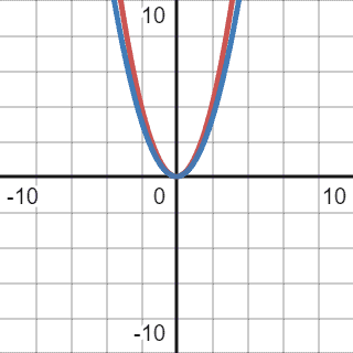
Visually, it’s represented by the graph below:
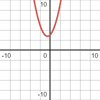
First of all, we should simplify the function. We should drop all the lower order components as they won’t significantly change when n approaches big values. For example, if we assume n as  , the equation will look like this:

The second and the third components will comprise a dramatically small part of the overall result. Thus we can drop them. Sometimes, it’s hard to define the higher-order component in more complex functions. Reference this table in case of any doubts.
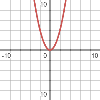
After simplification, we can reduce the function to  . Thus, the previous graph will change a bit, and the final version will be:
3.3. Big O Graphical Representation
As we already defined, the Big O notation represents the worst-case scenario. It will be a function higher than our function from a specific  to infinity.
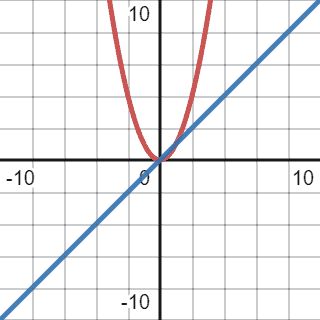
Let’s make a faulty assumption and decide to use a linear function for Big O notation:
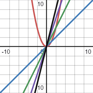
We compared our quadratic function with several linear: ,  ,
,  , and
, and  . However, because a quadratic function’s growth rate is greater than linear, it’s impossible to cap it with linear. Also, we used a constant multiplier for a function because we’re interested in the rate of growth which depends on the input. A constant, in this case, won’t make any difference.
Before checking the right solution, we can try another one that won’t work. We can try to cap our current quadratic function with a cubic one:

We can see overlapping graphs below:
As we can observe, cubic function caps quadratic function from 1 to infinity. We don’t care if the quadratic function, in this case, always has a higher value when  . Therefore, the cubic function completely fits the definition. However, we also should consider the tightness of the function, and in this case, the cubic function overshoots a lot. The comparison function should be as close to the given function as possible. Despite meeting all the requirements, we cannot use it to define complexity.
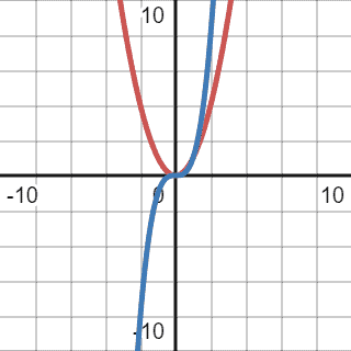
Let’s try to cap this function with a quadratic one:

The red graph represents our initial function, and the blue one represents the comparison function:
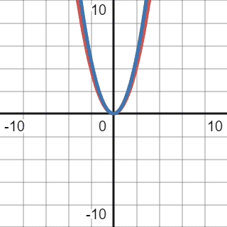
As we can see from the graph, the blue line representing our comparison function is always above our initial function. That’s why we can use this function for Big O notation. We should drop the constant multiplier as we’re only interested in the growth rate, not a specific value.
Thus, the Big O of our initial code block will be  . In most cases, the Big O of an equation will be the highest order component with all the constant multipliers dropped.
It is worth repeating that the comparison function should be as tight as possible to the function we want to estimate.
4. Big (Omega)
After learning about Big O notation, Big  should be easier to grasp. This asymptotic notation represents a lower bound of a given function. It means the best-case scenario for a function or an algorithm. However, considering that the function should be as tight as possible, we cannot go too optimistic.
Let’s consider the example from the beginning:
algorithm SortAndPrint(list):
    // INPUT
    //   list = A list of elements
    // OUTPUT
    //   Sorts the list, prints each element, and writes the list to a file
    bubbleSort(list)
    for element in list:
        print(element)
    writeToFile(list)
The complexity of this function is quadratic and, after simplification, will look the same as in the first example:
The best-case scenario is when all the elements are sorted already, and bubble sort will only go through the list once. Thus, we can assume that, theoretically, the best-case scenario will have linear complexity:
However, as mentioned before, even though this comparison function meets all the criteria, it’s not tight enough. We cannot assume that all the elements in a given list will be sorted in all the cases in real life. That’s why we need to find a function that will be as tight as possible to the current one:
The correct Big for the given code will be of quadratic complexity,  .
.
5. Big (Theta)
Big notation is the combination of both above. For the Big  , we need to use the function that perfectly fits the given function. To simplify, Big can be described as some function that, with the use of constant multipliers, can represent Big O and Big at the same time:
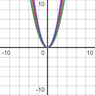
Two quadratic functions with different constant multipliers (0.8 and 1.2, respectively) contain inside the given function. Thus, the Big will also be of quadratic complexity.
6. Conclusion
This article taught us about asymptotic notations and why they are essential and valuable in computer science. Even a basic understanding of their use can help create better software.
These notations also help to think about algorithms in terms of efficiency and complexity. Even though modern machines’ hardware and computing power increased dramatically, so did the datasets these machines operate on. In most cases, it’s enough to concentrate on Big O notation for the accessing algorithms.
We can find a more practical look at this topic implemented in Java as well.